Tavernia

Forestry & Natural-Resource Sciences Last Correction: Aug. 15, 2013

CHANGES IN FOREST HABITAT CLASSES UNDER

ALTERNATIVE CLIMATE AND LAND-USE CHANGE

SCENARIOS IN THE NORTHEAST AND MIDWEST, USA

Brian G Tavernia

, Mark D Nelson

, Michael E Goerndt

,

Brian F Walters

, Chris Toney

1

Department of Biology, North Carolina State University, Raleigh, NC, USA

2_{USDA Forest Service, Northern Research Station, Saint Paul, MN, USA} 3_{Department of Forestry, University of Missouri, Columbia, MO, USA} 4_{USDA Forest Service, Rocky Mountain Research Station, Missoula, MT, USA}

Abstract. Large-scale and long-term habitat management plans are needed to maintain the diversity of

habitat classes required by wildlife species. Planning efforts would benefit from assessments of potential

climate and land-use change effects on habitats. We assessed climate and land-use driven changes in

areas of closed- and open-canopy forest across the Northeast and Midwest by 2060. Our assessments

were made using projections based on A1B and A2 future scenarios developed by the Intergovernmental Panel on Climate Change. Presently, forest land covers 70.2 million ha and is evenly divided between closed- and open-canopy habitats. Projections indicated that total forest land would decrease by 3.8 or 4.5 million ha for A2 and A1B, respectively. Within persisting forest land, the balance between closed and open-canopy habitats depended on assumed harvest rates of woody biomass. Standard harvest rates led to closed-canopy habitat attaining a slight majority of total forest land area. Intensive harvest rates resulted in the majority of forest land being in open-canopy habitat for A1B or maintained the even split between closed- and open-canopy habitats for A2. Ultimately, managers need to identify benchmark habitat conditions informed by historical conditions and wildlife population dynamics and plan to meet these benchmarks in dynamic forest landscapes.

Keywords: Wildlife Habitat; Bioenergy; Biomass Harvest; Climate Change; Young Forest; Early

Successional Habitat; FIA; Forest Projections.

1

Introduction

A significant challenge in natural resources manage-ment is providing sufficient habitat for wildlife species that have diverse and sometimes conflicting habitat needs (Magules and Pressey, 2000; Noon et al., 2009). Suites of species are associated with particular forest habitat classes characterized by different compositions, ages, and structures (Hagan et al., 1997; Patton, 2011).

For example, some species (e.g., Cerulean warbler,

Se-tophaga cerulea) are associated with mature,

decidu-ous forests whereas others (e.g., Kirtland’s warbler,

Se-tophaga kirtlandii) are found in disturbance-dependent early successional, coniferous habitat. Successful conser-vation and management of species with different habitat associations requires management plans that are large-scale and long-term in scope; such plans are necessary

to ensure that diverse habitat needs are simultaneously met and maintained through time (Hamel et al., 2005). Changing climate and land-use conditions are ex-pected to drive, in part, the large-scale dynamics of forest habitat and wildlife distributions over the com-ing decades and centuries (Iverson and Prasad, 1998; Matthews et al., 2004; Schwartz et al., 2006). Ecologists have long recognized large-scale associations between distributional limits of forest types and wildlife and cli-mate conditions (Booth, 1990; Newton, 2003; Prentice et al., 1992). As climate changes, some forest ecosystems and forest-associated species might shift their distribu-tions to track hospitable climate condidistribu-tions, and others might adapt to new climates (Iverson and Prasad, 1998; Matthews et al., 2004; Parmesan, 2006). When forest ecosystems and forest-associated species are unable to Copyright©2013 Publisher of theMathematical and Computational Forestry & Natural-Resource Sciences

move or adapt, their geographic ranges may shrink, or they may become extirpated from portions of their for-mer range (Parmesan, 2006; Thomas et al., 2004). To aid long-term conservation and management planning, researchers often model the potential distributions of for-est types and wildlife species under alternative climate change scenarios (Iverson and Prasad, 1998; Matthews et al., 2004; Schwartz et al., 2006). The direction and magnitude of modeled distributional changes are often scenario-specific, and accounting for uncertainty caused by scenario selection is a significant challenge (Beaumont et al., 2008).

Within large-scale patterns established by climate, land-use decisions further modify the extent and con-figuration of forest types and wildlife species diversity (Opdam and Wascher, 2004; Pearson et al., 2004). For-est conversion (e.g., to urban lands) reduces forFor-est area and potentially fragments forest ecosystems; this can re-sult in small, extirpation-prone wildlife populations that are too isolated to be rescued or re-established by immi-grants from the surrounding landscape (Robinson and Wilcove, 1994; Verboom et al., 1991). Land-use con-version may also place remaining forest habitat in close proximity to anthropogenic land-uses, including agricul-tural and urban areas. This proximity can alter food availability, ecological processes, and biotic interactions in ways that hasten the decline of wildlife populations (e.g., via increased nest predation pressure, Donovan et al., 1995). Researchers and managers recognize the im-portance of simultaneously assessing climate and land-use change effects (Pearson et al., 2004). Despite this, few such assessments exist due, in part, to a lack of climate and land-use projections that share common assumptions about future demographic, economic, and technological conditions (Bierwagen et al., 2010).

Quantity and quality of habitat can be affected by increases in woody biomass utilization for bioenergy. Woody biomass currently accounts for the greatest share of bio-energy generation in the U.S. at about 53% (U.S.

Energy Information Administration, 2012). Annual

woody biomass consumption for electricity generation is projected to increase over the next 20 years (U.S. En-ergy Information Administration, 2012). EnEn-ergy mar-kets for woody biomass may lead to the harvesting of stands previously viewed as being non-commercial (e.g., due to poor wood quality) and to shorter rotation times between harvests (Janowiak and Webster, 2010). For-est harvFor-est can increase the area of early successional or young forest habitat, benefiting wildlife dependent on this habitat (e.g., Annand and Thompson, 1997).

Plan-tations of short-rotation woody crop species (e.g.,Salix,

Populus) might serve as a source of biomass, and planta-tion establishment may have negative or positive effects on wildlife, depending on the land-use type that is

con-verted. Studies have generally found that plantations support fewer species of wildlife than unmanaged for-est (Moore and Allen, 1999), but the conversion of non-forest land-use types (e.g., agricultural fields) to planta-tions might benefit forest wildlife by increasing total area and connectivity of habitat (Cook and Beyea, 2000). Ul-timately, the value of plantations to wildlife species de-pends on how they are managed (Hartley, 2002).

Energy markets for woody biomass may also provide sufficient incentives to remove small-diameter woody material in addition to processing logging residues. In-tegrated harvest, which includes removal of both log-ging residues and small diameter trees, is one of sev-eral biomass procurement regimes that may be used to supply woody biomass for co-firing in electrical plants (Aguilar et al., 2012). The removal of woody residue previously left behind might negatively affect the abun-dance or quality of important microhabitat features, including downed woody material and snags, and the wildlife that depend on them, although more research

is needed (Riffell et al., 2011). These concerns have

led to several states adopting Best Management Prac-tices (BMPs) specifically designed to minimize impacts of woody biomass removal on water quality, soils, bio-diversity and wildlife habitat (Shepard, 2006; Skog and Stantkurf, 2011).

cur-rent FIA data do not include estimates of tree canopy cover.

Multi-species management planning is often based on coarse-filter assessments of the structure, function, and composition of habitat mosaics (Noon et al., 2009; Schulte et al., 2006). The types and areas of coarse habi-tat classes in a region can be used to broadly define the amount of habitat potentially available to broad suites of species (Beaudry et al., 2010). As part of the NFFP effort, we used projections of forest conditions in 2060 and ancillary data sets to assess potential changes in areas of forest habitat classes. The primary objective of this study was to assess potential changes to wildlife habitat classes over time under a suite of future sce-narios assuming different trajectories for climate, land-use, and biomass utilization. We defined our habitat classes using thresholds in canopy cover, providing us with the ability to crosswalk our habitat classes to a wildlife-habitat matrix created by NatureServe and to report species richness by taxonomic group and conser-vation status for each class.

2

Methods

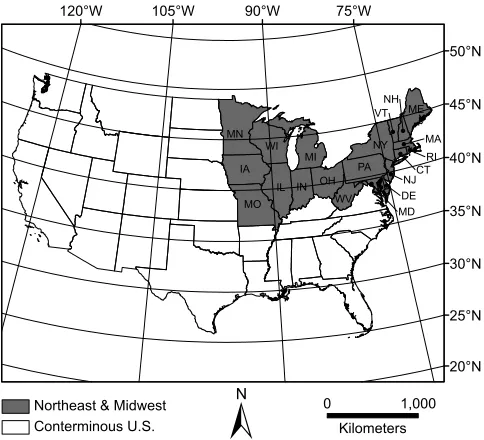
2.1 Region of Interest Our study area encompasses

the USDA Forest Service’s Eastern Region (Fig. 1). The Eastern Region is heavily forested relative to the whole U.S. (42% vs. 33%, respectively) and contains 32% of the nation’s timberland (Shifley et al., 2010). Approxi-mately 5 million private forest owners hold the majority (55%) of the region’s forest land and mostly adopt a low intensity management approach to their lands. The region supports 124 million people (41% of U.S. popu-lation) who depend on forests to supply a wide variety of ecosystem services (Shifley et al., 2010). Among a variety of forest resource issues, stakeholders in the re-gion are concerned about the ability of forest habitat to support diverse wildlife communities (Dietzman et al., 2011).

Well-informed forest and policy management decisions depend on assessments of the potential effects of alterna-tive decisions on a suite of forest resources and services. As part of the 2010 Forest and Rangeland Renewable Resources Planning Act (RPA) Assessment, the USDA Forest Service used alternative future scenarios of cli-mate change, land-use change, and human population growth (described below) to project forest and rangeland conditions in 2060 for the Eastern Region (USDA For-est Service, 2012a). We used FIA data (described below) to estimate current conditions and to project potential future forest conditions. We applied alternative RPA scenarios to project potential changes in forest habitat classes needed to sustain regionally diverse wildlife com-munities.

MO IL

75°W 90°W

105°W 120°W

50°N

45°N

40°N

35°N

30°N

25°N

20°N

0 1,000

Kilometers

IA MN

WI

IN MI

OH PA

NY VT NH

ME

MA

RI CT NJ DE MD WV

Northeast & Midwest Conterminous U.S.

Figure 1: Map showing the location of states across the Northeast and Midwest, USA, an area corresponding to the USDA Forest Service’s Eastern Region. States in-clude: Connecticut (CT), Delaware (DE), Illinois (IL), Indiana (IN), Iowa (IA), Maine (ME), Maryland (MD), Massachusetts (MA), Michigan (MI), Minnesota (MN), Missouri (MO), New Hampshire (NH), New Jersey (NJ), New York (NY), Ohio (OH), Pennsylvania (PA), Rhode Island (RI), Vermont (VT), West Virginia (WV), and Wisconsin (WI).

2.2 FIA Data FIA’s definition of forest land includes

a plot contains a forest land use (Bechtold and Scott, 2005; Reams et al., 2005). FIA began collecting tree canopy cover data only recently; such data are absent from historical FIA inventories.

FIA data from 2004-2008 were used to produce es-timates of current conditions, assigned the decadal la-bel of ‘2010’ and referred to as ‘baseline’. These same FIA data were also used to model future projections, by decade, as described below. Estimates of baseline and future conditions were produced using estimators within PC-EVALIDator tools in the Northern Forest Futures Database (NFFDB) (Miles et al., 2013).

2.3 Future Scenarios The RPA Assessment used

climate (Coulson and Joyce, 2010; Coulson et al. 2010), land-use (Wear, 2011), and population (Zarnoch et al., 2010) projections consistent with greenhouse gas emission scenarios developed by the Intergovernmental Panel on Climate Change (IPCC) (USDA Forest Service, 2012a). The analyses by RPA represented an adaptation of the broad IPCC scenarios to a regional-scale through downscaling of climate change, economical, and popu-lation projections (USDA Forest Service, 2012a; USDA

Forest Service, 2012b; Wear et al., 2013). Emissions

scenarios were consistent with IPCC storylines that as-sumed different trajectories of change for global popu-lations and gross domestic product (Tab. 1). For the RPA Assessment, the USDA Forest Service elected to use IPCC’s A1B, A2, and B2 storylines because these captured a range of potential futures likely to drive vari-ation in natural resources (USDA Forest Service, 2012a). These storylines also had marker emission scenarios that used common assumptions about driving forces in rylines, were intended to illustrate their respective sto-rylines, and were subjected to greater scrutiny (USDA Forest Service, 2012a). While capturing a range of po-tential futures, these storylines are not tied to specific policy or management actions. We chose to use emission scenarios from the A1B and A2 storylines for our forest

habitat assessments. We eliminated the B2 storyline

because recent observations of greenhouse gas emissions (Raupach et al., 2007) suggest that projected emissions under this storyline may underestimate actual emissions. There are many sources of uncertainty when assessing future changes in natural resources conditions (Beau-mont et al., 2008). The A1B and A2 storylines capture some uncertainty by representing a range of likely future climate, land-use, and population conditions. Projected changes in climate for each storyline’s emission scenario depend on the general circulation model (GCM) used to simulate future climate conditions. For the RPA, the USDA Forest Service projected future climate change us-ing projections from three GCMs: CGCM 3.1 MR (T47) developed by the Canadian Centre for Climate

Model-Table 1: Projections of global population and global gross domestic product (GDP) associated with Intergov-ernmental Panel on Climate Change storylines. Source: USDA Forest Service (2012a).

Storyline 2010 2020 2040 2060

Global Population (millions)

A1 6,805 7,493 8,439 8,538

A2 7,188 8,206 10,715 12,139

B2 6,891 7,672 8,930 9,704

Global GDP (2006 trillion USD)

A1 54.2 80.6 181.8 336.2

A2 45.6 57.9 103.4 145.7

B2 67.1 72.5 133.3 195.6

ing, and Analysis; CSIRO MK 3.5 (T63) developed by Australia’s Commonwealth Scientific and Industrial Re-search Organization; and MIROC 3.2 MR (T42) devel-oped jointly by Japan’s National Institute for Environ-mental Studies, Center for Climate System Research, University of Tokyo, and Frontier Research Center for Global Change. These GCMs had average or above av-erage sensitivity to greenhouse gas emissions (Randall et al., 2007), showed a reasonable degree of accuracy when simulating present-day mean climate conditions (Reich-ler and Kim, 2008), and produced a range of future cli-mate conditions. To address uncertainty resulting from choice of IPCC storylines and GCMs, we assessed po-tential changes of forest habitat conditions in 2060 un-der six scenarios representing unique combinations of A1B and A2 IPCC storylines and CGCM, CSIRO, and MIROC GCMs. Table 2 summarizes projected changes in climate, land-use, and population under each scenario. Maps of current and projected changes in climate con-ditions can be found in Tavernia et al. (2013).

2.4 Forest Projections Estimation of future forest

ma-jor forest type group was assigned based on forest type, ii) variables for physical characteristics (slope, aspect, etc.) were retained, and iii) biophysical attributes (basal area, growing stock volume, number of trees, etc.) at the population (expanded) and per-acre scale were cal-culated. Transition, partitioning, and imputation sub-models were used to predict change in forest plot condi-tions through time.

The transition submodel projects changes in forest type, forest age, and harvesting and the exogenous cli-mate models project changes in key clicli-mate variables. The transition submodel selects a specific outcome (con-dition) from among all possible outcomes through com-binations of forest type, forest age, harvest history and climate variables represented in a probability matrix. The partitioning submodel groups plots from the 2010 baseline record (we call these donor plots) based upon a set of biophysical attributes. The plot characteristics that defined the partitioned groups included forest at-tributes such as stand age, slope, and ownership, as well as climate variables such as average temperature and precipitation. Given the conditions for each future plot, the imputation submodel draws a random donor plot (with replacement) from the plot’s appropriate group as defined by the partitioning submodel. For example, if the transition probabilities state that a 50-year-old oak-hickory plot will become a 55-year-old oak-oak-hickory plot (instead of an elm-ash-cottonwood plot or some other forest type group), then the model imputes what this 50-year-old plot will look like in five years by randomly picking an oak-hickory plot from the group of existing 55-year-old plots that have similar ecological characteris-tics. The time step for imputation was set as the span of years between re-measurements for individual FIA plots. Hence, the time step for imputation in the Northcentral and Northeast states was five years (Wear et al., 2013). FDM projections were validated by applying the model to past FIA inventories for select states and comparing the projections to present-day FIA inventories. Addi-tionally, calibrations were made to the FDM at the state-level following reviews by USDA Forest Service FIA and state foresters and planners to account for past trends in forest change (Moser and Shifley, 2012; Wear et al., 2013).

The transition and imputation submodels used proba-bilistic (Monte Carlo) methods to simulate variance as-sociated with different model components. Note that the algorithm for the imputation submodel was run 26 times with random selection for donor plots in each time step resulting in 26 “inventories”. The stochastic nature of the imputation model implies that no two invento-ries were exactly alike. Aggregate validation was per-formed by comparing 95% confidence intervals for trees per acre, total biomass, and sawtimber biomass for both

hardwoods and softwoods using all 26 inventories (Wear et al., 2013). Ultimately, only one inventory was used to estimate forest attributes for each future scenario in the NFFDB. The selected inventory was the one with the greatest “central tendency,” defined as minimum pro-portional distance of total growing stock volume, trees per acre and sawtimber volume for softwoods and hard-woods from their means over the 50-year projection pe-riod (Wear et al., 2013). The completed database sum-marizes the results of the FDM for future decades by summarizing plot conditions for a projected future date in the same way that one would summarize current or past forest conditions (Miles, 2013).

Projections of forest conditions for combinations of IPCC storylines and CGCM included variations which accounted for higher assumed increases in woody biomass utilization in the future. While not tied to spe-cific forest management policies, these alternative sce-narios (designated as “BIO” scesce-narios) show substan-tial growth in harvesting reflecting the expansion in de-mands for forest biomass in bioenergy production associ-ated with each scenario. These expansions were applied to the scenarios by adjusting harvest probabilities to re-flect the harvests predicted by the U.S. Forest Products Model (Ince et al., 2011). Probability of harvest was ad-justed for these scenarios in the FDM by increasing the probability of harvest by a pre-determined percentage via a scale parameter. Consequently, for each BIO sce-nario, the probability of harvest was increased by the

same proportion across the region. Note that global

assumptions regarding plantation woody biomass were included in the RPA projections; however, plantation biomass does not play a significant role in the projec-tions from the FDM (Ince et al., 2011; USDA Forest Service, 2012a). Harvest projections for the BIO sce-narios deviated from the original scesce-narios starting in 2020 for the A1B and A2 storylines. For the A1B-BIO storyline, harvest levels were projected to reach approx-imately 3 times the 2010 level by 2060. Similarly, for the A2-BIO storyline, harvest levels were projected to be roughly 2.5 times the 2010 level by 2060 (Wear et al., 2013).

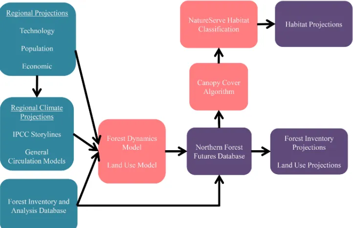
Figure 2: Modeling process used to project changes in the areas of forest habitat classes by 2060. Population, technological, economic, and climate projections served as input to Forest Dynamics and Land Use Models and drove changes in the extent and composition of forests from 2010 to 2060 at 5-year increments. Input projections represented future scenarios resulting from the combination of Intergovernmental Panel on Climate Change (IPCC) storylines and General Circulation Models. Data and trends from the USDA Forest Service’s Forest Inventory and Analysis Database established 2010 forest conditions and informed projections of forest change out to 2060. Projected land-use conditions and forest inventories were summarized in the Northern Forest Futures Database (NFFDB). A canopy cover algorithm assigned canopy cover estimates to forested conditions in the NFFDB, enabling forest projections to be translated into forest habitat classes found within a NatureServe habitat classification system. Green nodes represent input data, pink nodes indicate modeling steps, and purple nodes are output products. Flowchart adapted from Wear et al. (2013).

allocation of rural land (land not converted to urban) was greatly based on the existing distribution of different non-urban land classifications from historical data. All federal land, water area, enrolled Conservation Reserve Program lands, and utility corridors were held constant for all projections (Wear, 2011).

Output from the forest projection process described above was combined with data from the FIADB (Woudenberg et al., 2010) to produce the NFFDB (Fig. 2) (Miles, 2013; Miles et al., 2013).

2.5 Habitat and Species Richness Assessments

Within the NFFDB, we assigned FIA forested condi-tions to six different habitat classes defined to match classes in a wildlife-habitat matrix created by Nature-Serve (2011) and purchased by the USDA Forest Ser-vice for the NFFP (Tab. 3). Using canopy cover thresh-olds, we arrayed habitat classes along two dimensions ad-dressing differences in structure and composition. With respect to structure, we identified classes as being

ei-ther closed- (>66% total canopy cover) or open-canopy

(10 to 66%). Our closed-canopy definition is consistent with NatureServe’s (2011) definition of ‘forest’ habitat class whereas our open-canopy definition encompasses both NatureServe’s ‘woodland’ (40 to 66% canopy cover) and ‘savanna’ (10 to 40% canopy cover) habitat classes. Following consultation with NatureServe staff (J. Mc-Nees, pers. comm., NatureServe, December 19, 2011), we included NatureServe ‘savanna’ in our open-canopy class because regenerating forest with sparse canopy is not synonymous with a savanna ecosystem, and because actual savanna habitat is very rare in our study area. To avoid confusion with FIA’s definition of forest land, which encompasses all three NatureServe (2011) habitat classes – ‘forest’, ‘woodland’, and ‘savanna’, we refer to closed- and open-canopy habitat classes. Closed- and open-canopy classes were further refined based on dif-ferences in composition. We labeled areas as hardwood

or conifer when>66% of the canopy consisted of

Table 2: Mean monthly temperature (T) and precipitation (PPT), land-use conditions (%), and population under baseline conditions and six future scenarios for the Northeast and Midwest, USA. Future scenarios were defined using unique combinations of Intergovernmental Panel on Climate Change storylines and General Circulation Models (GCM). Mean climate conditions were calculated using area-weighted means of county-level values. Baseline and future climate data from Coulson and Joyce (2010) and Coulson et al. (2010), land-use from Wear (2011), and population projections from Zarnoch et al. (2010).

Storyline GCM T (◦C) PPT (mm) Urban Forest Crop Pasture Population (mill.)

Baseline Historical 9.1 80.5 9.4 41.4 39.3 9.9 124.1

A1B CGCM 11.4 84.4 15.5 38.7 36.5 9.3 157.6

CSIRO 11.5 79.8 15.5 38.7 36.5 9.3 157.6

MIROC 13.1 72.6 15.5 38.7 36.5 9.3 157.6

A2 CGCM 11.8 83.1 14.2 39.2 37.2 9.4 178.0

CSIRO 11.2 86.2 14.2 39.2 37.2 9.4 178.0

MIROC 12.4 75.0 14.2 39.2 37.2 9.4 178.0

cover exceeds 66% of the total canopy cover, consistent with NatureServe’s definitions.

Using the NatureServe matrix, we tabulated numbers of terrestrial vertebrate species within the study area, by major taxon (amphibians, birds, mammals, reptiles) associated with each of six habitat classes, and by global rank (NatureServe, 2011). Habitat associations reflected species’ entire annual cycles, i.e., a species could be as-sociated with a habitat type during any season. Rank is defined as follows: 1 = critically imperiled; 2 = im-periled; 3 = vulnerable to extirpation or extinction; 4 = apparently secure; 5 = demonstrably widespread, abun-dant, and secure. A small number of records had “T” ranks (infraspecific taxon: subspecies or varieties); these were combined with “G” ranks (global ranks), and all re-sults were labeled as ranks (G1-G5). For the purposes of our coarse-filter assessment, we summarized numbers and global ranks to characterize wildlife communities that might be affected by projected changes in habitat classes. Projections of changing habitat associations or global ranks for individual species fell outside the scope of our study. Such species-specific assessments might be important and appropriate if the objective is to inform species-level conservation objectives, but our assessment focused on changes in coarse habitat classes.

FIA does not provide estimates of canopy cover, so we used a computer algorithm to derive estimates of canopy cover from FIA data, enabling us to crosswalk NFFDB area projections to habitat classes (Fig. 2). A canopy cover modeling approach (Toney et al., 2009) was used

to estimate canopy cover for trees (> 5 in. d.b.h., on

subplots), if present, or saplings (1-4.9 in. d.b.h., on microplots) on forested FIA conditions within 20 states of USDA Forest Service’s Eastern Region, during the

inventory period 2004-2008. Canopy cover estimation was based on tree species-specific predicted crown di-mensions, and tree stem location coordinates recorded by field crews within FIA subplots and microplots. Tree and sapling crown width predictions are based on Bech-told (2003) and Bragg (2001). An optional spatial statis-tic (Ripley’s K) included as a predictor in Toney et al. (2009) was not utilized for canopy cover modeling in the present study. Because FIA plots may contain multiple conditions, tree and sapling canopy cover estimates were weighted based on condition proportion and appended to the CONDITION table in the NFFDB.

Table 3: Forest habitat classes (adapted from NatureServe Habitat Classes, 2011).

Class Name NatureServe

Habitat Class

Description

Closed-canopy forest

Forest Woody vegetation at least 6 m tall (usually much taller) with a fairly

con-tinuous and complete (two-thirds or greater) canopy closure. Closed-canopy

hardwood

Forest-hardwood

Angiosperms comprise over two-thirds of the canopy.

Closed-canopy conifer

Forest-conifer Gymnosperms comprise over two-thirds of the canopy.

Closed-canopy mixed

Forest-mixed Composed of both hardwood and conifer trees, neither dominating as much

as two-thirds of the canopy. Open-canopy

forest

Woodland & Sa-vanna

Crowns often not interlocking; tree canopy discontinuous (often clumped), averaging between 40 and 66 percent overall cover (Nature Serve Wood-land), or, mosaic of trees or shrubs and grassland; between 10 and 40 percent cover by trees and shrubs (Nature Serve Savanna).

Open-canopy hardwood

Woodland-hardwood

Angiosperms comprise over two-thirds of the canopy.

Open-canopy conifer

Woodland-conifer

Gymnosperms comprise over two-thirds of the canopy.

Open-canopy mixed

Woodland-mixed

Stand composed of both hardwood and conifer trees, neither dominating as much as two-thirds of the canopy.

3

Results

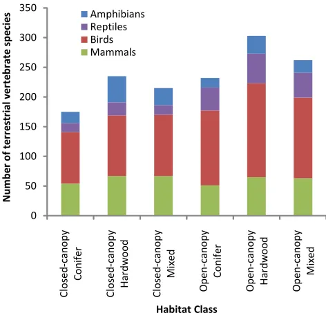
Birds were the most numerous terrestrial vertebrate species associated with closed- or open-canopy forest habitat classes within the study area at 189 species, fol-lowed by mammals (85), reptiles (52), and amphibians (50). For every one of the six individual habitat classes, birds and mammals had most species (Fig. 3). Am-phibian species outnumbered reptiles in all three closed-canopy classes; reptile species outnumbered amphibians in all three open-canopy classes (Fig. 3).

Overall, 25 of 376 species (6.6%) were listed within one of the three most at-risk ranks (G1-G3), ranging from a low of 1.1% for birds, to a high of 14.1 % for mammals. Amphibians and reptiles were intermediate, with 12.0% and 9.6%, respectively. Figure 4 presents numbers of species by global rank within each habitat class. The habitat classes with highest and lowest percentages, re-spectively, of at-risk species (G1-G3) were closed-canopy hardwood (7.3%), and open-canopy mixed (1.9%). Note that many species were associated with multiple habitat classes, so it is not valid to sum species counts across habitat classes in Figure 3 or 4.

Per-plot estimates of canopy cover were used to assign habitat classes. Because almost all FIA forested condi-tions were assigned habitat labels, total area of habitat classes was essentially equivalent to FIA forest land area for the study area (Nelson et al., 2012). Mean canopy cover of forest land across the study area was 60.4%, ranging from lows of 41.6 – 55.3% in Minnesota, Maine,

0 50 100 150 200 250 300 350 C lo se d -c a n o p y C o n if e r C lo se d -c a n o p y H a rd w o o d C lo se d -c a n o p y M ix e d O p e n -c a n o p y C o n if e r O p e n -c a n o p y H a rd w o o d O p e n -c a n o p y M ix e d N u m b e r o f te rr e st ri a l v e rt e b ra te s p e ci e s Habitat Class Amphibians Reptiles Birds Mammals

Figure 3: Number of terrestrial vertebrate species asso-ciated with closed- and open-canopy conifer, hardwood, and mixed forest, Midwest and Northeast USA, by ma-jor taxon. (Adapted from NatureServe, 2011)

Wisconsin and Michigan, to highs of 74.2 – 75.8% in Rhode Island, Massachusetts, and Connecticut.

Table 4: Area (millions of ha) and percent change of six closed- (CC) and open-canopy (OC) forest habitat classes across the Northeast and Midwest. Estimates are provided for 2010 baseline conditions and for six 2060 scenarios representing unique combinations of two Intergovernmental Panel on Climate Change storylines (IPCC) and three General Circulation Models (GCM). Two 2060 scenarios assuming intensive biomass utilization for bioenergy (A1B-BIO, A2-BIO) are also included. Changes in habitat classes between 2010 and 2060 were driven by projected climate and land-use changes, forest succession, and forest harvest. See Table 3 for explicit definitions of forest habitat classes.

IPCC GCM Total

Habitat CC Hard-wood CC Conifer CC Mixed OC Hard-wood OC Conifer OC Mixed

Baseline Historical 70.2 28.5 1.7 4.4 24.1 6.7 4.7

A1B-BIO CGCM 65.7

(-6.4%) 22.8 (-20.0%) 1.4 (-17.6 %) 3.2 (-27.3%) 27.6 (14.5%) 6.4 (-4.5%) 4.4 (-6.4 %)

A1B CGCM 65.7

(-6.4%) 29.6 (3.9%) 2.1 (23.5%) 4.6 (4.5%) 19.6 (-18.7%) 5.8 (-13.4%) 4.0 (-14.9%) CSIRO 65.7 (-6.4 %) 29.5 (3.5%) 2.0 (17.6%) 4.7 (6.8%) 19.6 (-18.7 %) 5.8 (-13.4%) 4.2 (-10.6%) MIROC 65.7 (-6.4%) 29.4 (3.2%) 2.1 (23.5%) 4.5 (2.3 %) 19.7 (-18.3%) 5.8 (-13.4%) 4.3 (-8.5%)

A2-BIO CGCM 66.4

(-5.4%) 26.4 (-7.4%) 1.6 (-5.8%) 3.9 (-11.4%) 24.0 (-0.4%) 6.2 (-7.5%) 4.4 (-6.4%)

A2 CGCM 66.4

(-5.4%) 30.1 (5.6%) 2.0 (17.6%) 4.7 (6.8 %) 19.7 (-18.3%) 5.9 (-11.9%) 4.1 (-12.8%) CSIRO 66.4 (-5.4%) 29.9 (4.9%) 2.0 (17.6%) 4.6 (4.5 %) 19.8 (-17.8%) 5.8 (-13.4%) 4.3 (-8.5%) MIROC 66.4 (-5.4 %) 29.9 (4.9%) 2.0 (17.6%) 4.7 (6.8%) 19.9 (-17.4 %) 5.9 (-11.9%) 4.0 (-14.9%) 0 50 100 150 200 250 300 350 C lo se d -c a n o p y C o n if e r C lo se d -c a n o p y H a rd w o o d C lo se d -c a n o p y M ix e d O p e n -c a n o p y C o n if e r O p e n -c a n o p y H a rd w o o d O p e n -c a n o p y M ix e d N u m b e r o f te rr e st ri a l v e rt e b ra te s p e ci e s Habitat Class G1 G2 G3 G4 G5

Figure 4: Number of terrestrial vertebrate species as-sociated with closed- and open-canopy conifer, hard-wood, and mixed forest, Midwest and Northeast USA, by global rank. (Adapted from NatureServe, 2011)

Of 0.6 million ha in nonstocked conditions, 0.3 million ha were assigned to habitat classes and 0.3 million ha were omitted from the habitat classification (0.4% of total forest land area), resulting in 70.2 million ha assigned to six habitat classes (Tab. 4). The region is dominated by the closed-canopy hardwood (40.6% of forest habitat) and open-canopy hardwood (34.3%) habitat classes with no other class exceeding 10% of forest habitat. Forest land is approximately evenly split between the groups of closed- and open-canopy habitat classes (49.3% and 50.7%, respectively).

pro-cess, all subsequent results are reported only for per-state or region-wide scales.

Assuming standard forest harvest levels, loss of habi-tat area was projected under both IPCC storylines with the magnitude of loss ranging from 3.8 million ha (5.4%) under A2 to 4.5 million ha (6.4%) under A1B (Tab.

4). While projected losses for total habitat area did

not differ among GCMs for either storyline, choice of GCM did affect projected changes for individual habi-tat classes, but these effects were relatively minor and

varied across habitat classes. For example, areas for

the open-canopy mixed habitat class ranged from 4.0 (CGCM) to 4.3 million ha (MIROC) whereas areas for open-canopy conifer did not vary under the A1B story-line. Patterns of change for habitat classes were con-sistent across both IPCC storylines (Tab. 4). All three closed-canopy forest habitat classes gained area; percent gains were greatest for closed-canopy conifer and least for either closed-canopy hardwood or mixed, depending on the GCM. Conversely, all three open-canopy habitat classes lost area; percent losses were greatest for open-canopy hardwood and least for open-open-canopy conifer or mixed, depending on the GCM. Closed-canopy habitat classes (54.7 to 55.3%) were projected to increase rela-tive to open-canopy habitat classes (44.7 to 45.3%) as a percent of total habitat regardless of the scenario con-sidered.

Under the high biomass utilization scenarios, loss of habitat area was projected under both IPCC

sto-rylines, with one exception: A1B-BIO-CGCM

open-canopy hardwood class gained 3.5 million ha (Tab. 4). Across the other eleven classes, A1B-BIO-CGCM closed-canopy mixed displayed the greatest percent loss, and A2-BIO-CGCM open-canopy hardwood displayed the least (Tab. 4). Thus, patterns of change were mostly consistent, but not in magnitude across IPCC storylines (Tab. 4). Under the A1B-BIO-CGCM scenario, closed-canopy habitat classes were in the minority (41.6% ver-sus 58.4% for open-canopy classes) whereas, under the A2-BIO scenario, the closed- and open-canopy classes remained relatively balanced (48.0% versus 52.0%, re-spectively).

The greatest spatial contrasts seen in Figure 5 pertain to states with well-established timber industries, such as Minnesota, Wisconsin, and Maine. These states showed general increases in forest land area for all closed canopy classes for the original scenarios, but displayed some of the greatest losses in closed canopy classes for the BIO scenarios.

4

Discussion

Adopting a coarse-filter approach, we used climate and land-use projections sharing a common set of

as-sumptions to assess potential changes in forest habitat classes across the Northeast and Midwest from 2010 to 2060. For all scenarios considered, our assessments sug-gest that the total area of forest habitat classes will de-crease, and this loss in total habitat area has the po-tential to negatively affect wildlife populations. For an individual species, the degree of these effects may de-pend, in part, on the spatial pattern of habitat loss. Although we do portray regional variation in habitat trends among states, we did not directly assess spatial patterns of habitat loss at a fine scale. Overall reduction in habitat area can lead to smaller and more isolated forest patches. These patches support fewer individu-als and are less likely to receive immigrants from other areas, increasing the likelihood of local extirpation and decreasing likelihood of recolonization or population res-cue (Hanski, 1999). Habitat in smaller forest patches in this region of North America is also more exposed to negative ecological influences (e.g., nest predators, Donovan et al., 1995) from surrounding non-forest land-uses, contributing to local population declines. Land-use and climate changes may have synergistic effects on species. For example, reduced connectivity among for-est patches might influence the ability of a species to locate and occupy climatically suitable environments as these shift in response to changing climate conditions (Hannah, 2008; Opdam and Wascher, 2004). If habi-tat loss is widespread, regional declines and extirpations may result.

Our assessments suggest that uncertainty about fu-ture demographic, economic, technological, and climate conditions (as represented by different IPCC-GCM sce-narios) contributes to uncertainty about the extent of habitat loss. While we did not quantify it, additional uncertainty arises from the unknowable possibility that future forest and land-use management actions might greatly depart from historically observed actions. Pol-icy (e.g., promoting growth near existing urban centers) and financial mechanisms (e.g., tax deductions result-ing from conservation easements) might be used to limit negative effects of land-use change on forest wildlife.

The number of terrestrial vertebrate species varied among major taxa and among closed- and open-canopy hardwood, conifer, and mixed forest habitat classes. Birds and mammals dominated species richness. The number of species at-risk rank was relatively low (6.6%), with the largest percentages observed for mammals and amphibians. While numbers of species were not pro-jected for future conditions, consideration for at-risk species may be needed for habitat classes projected to decline in future decades.

A1B-BIO A2-BIO

A1B A2

2010

C

lo

se

d

-C

a

n

o

p

y

H

a

rd

w

o

o

d

C

lo

se

d

-C

a

n

o

p

y

C

o

n

if

e

r

C

lo

se

d

-C

a

n

o

p

y

M

ixe

d

O

p

e

n

-C

a

n

o

p

y

H

a

rd

w

o

o

d

O

p

e

n

-C

a

n

o

p

y

C

o

n

if

e

r

O

p

e

n

-C

a

n

o

p

y

M

ixe

d

Percent Change (2010 - 2060)

< -25%

-25 - 0%

0 - 25%

> 25%

No Data Percent of Forest Land (2010)

0 - 1%

1 - 10%

10 - 25%

25 - 50%

> 50%

Figure 5: Percent change in area of closed- and open-canopy habitat classes, 2010-2060, by state and future scenarios. Percent of 2010 forest land area within each habitat class is shown for reference (left column). Future scenarios involved two Intergovernmental Panel on Climate Change storylines (A1B, A2) and the CGCM 3.1 MR (T47) general circulation model. Scenarios assumed either standard harvest rates (A1B, A2) or intensive harvest rates for high biomass utilization (A1B-BIO, A2-BIO).

have been attributed to a number of different causes including forest maturation of abandoned farmland, al-tered forest management practices, forest ownership pat-terns that discourage harvest, disrupted natural distur-bance regimes (e.g., fire suppression), and land-use con-version (Askins, 2001; Lorimer and White, 2003; Trani et al., 2001). Assuming that early successional forests can be characterized as having more open canopies, pro-jections of open-canopy habitat classes in our assessment suggested that declines of this habitat type may continue into the near future. With the exception of intensive biomass utilization scenarios, we found that all open-canopy habitat classes declined and that regional habi-tat became dominated by closed-canopy habihabi-tat classes. These projected declines may negatively affect not only

open-canopy associated species but also species typi-cally associated with closed-canopy habitats that depend upon open-canopy areas during certain times of the year (e.g., Streby et al., 2011; Vitz and Rodewald, 2006). Ultimately, the future status of wildlife species depen-dent on young forests or open-canopy habitat will de-pend on the scale, type, and frequency of anthropogenic and natural disturbances occurring in landscapes across the Northeast and Midwest.

as being non-commercial (e.g., due to poor wood qual-ity) and lead to shorter rotation times (Janowiak and Webster, 2010). Harvest of woody biomass has the po-tential to open up forest canopies and turn back succes-sion, influencing the balance between closed- and open-canopy habitat classes. Our intensive biomass utiliza-tion scenarios led to smaller decreases for open-canopy habitat classes relative to the other scenarios consid-ered; one class (open-canopy hardwood) even displayed an increase under the A1B-BIO-CGCM scenario. Under the intensive biomass utilization scenarios, the percent cover of forest land in the open-canopy habitat classes re-mained stable or increased relative to current conditions. This contrasts with our other scenarios in which percent cover of open-canopy habitat classes declined and the closed-canopy habitat classes attained a slight majority. Policies and tactics associated with woody biomass har-vest will partly determine the degree to which wildlife species dependent on open-canopy habitat classes might benefit. Biomass harvest for bioenergy might incentivize the removal of woody residue, or woody materials typ-ically left behind after harvest (e.g., tops, dead wood). These materials contribute to important microhabitat conditions that can influence the habitat quality of an area. Several states have adopted BMPs specifically de-signed to minimize impacts of woody biomass removal on water quality, soils, biodiversity and wildlife habitat (Shepard, 2006; Skog and Stantkurf, 2011). We did not examine changes in microhabitat features as a result of intensive biomass utilization due to limitations of avail-able FIA data and the projection technique.

Recall that some of the stark contrasts between the original scenarios and the BIO scenarios regarding canopy cover classes occurred in northern states with relatively high current levels of forest products utiliza-tion, such as Minnesota, Wisconsin, and Maine. This was greatly due to the high current probabilities of har-vest within these states resulting in greater increases in harvest probability within the FDM for the BIO

sce-narios. This is logical, as the probability of harvest

was increased by the same proportion across the region when the FDM was adjusted for higher biomass utiliza-tion (Wear et al., 2013). Consequently, many of these same states also show lower decreases (and sometimes in-creases) in forest area for the open canopy classes when compared to the original scenarios A1B and A2. While the variability in direction and magnitude of change among scenarios cautions against over-interpretation, these results suggest that future trends in forest habi-tat conditions will vary across shabi-tates presenting unique challenges to wildlife managers in different areas.

Interpreting the significance of projected shifts in the representation of closed- and open-canopy habitat classes is difficult without appropriate ecological

con-text. One viewpoint is that the historical balance be-tween closed- and open-canopy habitat classes should be the standard because these are the conditions un-der which organisms evolved (Askins, 2001; Litvaitis, 2003; Lorimer, 2001; Thompson and DeGraaf, 2001). Estimating the frequency and extent of historical dis-turbance events and open-canopy habitat is difficult for a variety of reasons, including difficulty differentiating natural from anthropogenic disturbances and spatiotem-poral variation in disturbance rates (Lorimer, 2001). To cope with temporal variability in disturbance rates, re-searchers have suggested managing habitat classes to maintain a balance that falls within the range of histor-ical variability (Thompson and DeGraaf, 2001). With respect to wildlife management, it is important to con-sider the minimal amount of open-canopy (or other habi-tat class) required to support viable populations (Ask-ins, 2001; Lorimer, 2001). Studies have indicated that species dependent on open-canopy habitat might re-spond to decreasing habitat areas in non-linear, thresh-old fashions although these threshthresh-olds might occur at relatively low levels of habitat cover (e.g., Betts et al., 2010). Identifying appropriate benchmarks for habitat management remains an active field of research.

It can be difficult to associate FIA data with habi-tat classes in established wildlife-habihabi-tat matrices. The method presented here provides an operational approach to predicting per-condition tree canopy cover from FIA tree data, with resulting classifications used to as-sign FIA conditions to closed- and open-canopy habitat classes, for which population estimates were produced. Although FIA’s forest land definition requires a min-imum of 10 percent canopy cover, a small area of FIA forest land was characterized by canopy cover below this threshold. Such conditions likely occur shortly after full canopy removal (e.g., harvest, wildfire, etc.), but be-fore regenerating seedlings have established significant canopy. Tree canopy cover predictions allowed FIA data to be used with NatureServe’s (2011) wildlife-habitat matrices to summarize species distribution across habi-tat classes. Because choice of habihabi-tat classification sys-tems can affect resulting estimates of habitat abundance, work continues to link FIA data with a variety of habi-tat classifications systems, including the National Veg-etation Classification System (Federal Geographic Data Committee, 2008).

and the balance between different habitat classes might shift in the future. The influence of assumptions about biomass utilization on the balance between closed- and open-canopy habitat classes highlights the importance of policy and management decisions in determining habi-tat conditions in the future. Ultimately, managers will need to identify benchmark habitat conditions informed by historical conditions and wildlife population dynam-ics and to develop plans to meet these benchmarks in dynamic forest landscapes.

Acknowledgements

The authors thank NatureServe for producing a ter-restrial vertebrate species-habitat matrix for forest-associated species. The authors also acknowledge the assistance of J.M. Reed, J. Stanovick, S. Oswalt, and three anonymous reviewers whose suggestions improved the manuscript.

References

Aguilar, F.X., M. Goerndt, N. Song, and S. Shifley. 2012. Internal, External and Location Factors Influencing Cofiring of Biomass with Coal in the U.S. Northern Region. Energ. Econ. 34:1790-1798.

Annand, E.M., and F.R. Thompson, III. 1997. For-est bird response to regeneration practices in central hardwood forests. J. Wildlife Manage. 61:159-171. Askins, R.A. 2001. Sustaining biological diversity in

early successional communities: the challenge of man-aging unpopular habitats. Wildlife Soc. B. 29:407-412. Beaudry, F., A.M. Pidgeon, V.C. Radeloff, R.W. Howe, D.J. Mladenoff, and G.A. Bartelt. 2010. Modeling regional-scale habitat of forest birds when lands man-agement guidelines are needed but information is lim-ited. Biol. Conserv. 143:1759-1769.

Beaumont, L.J., L. Hughes, and A.J. Pitman. 2008. Why is the choice of future climate scenarios for species distribution modeling important? Ecol. Lett. 11:1135-1146.

Bechtold, W.A. 2003. Crown-diameter prediction mod-els for 87 species of stand-grown trees in the Eastern United States. South. J. Appl. For. 27: 269-278. Bechtold, W.A., and C.T. Scott. 2005. The Forest

In-ventory and Analysis plot design. P. 27-42 in The Enhanced Forest Inventory and Analysis Program – National Sampling Design and Estimate Procedures. W.A. Bechtold and P.L. Patterson (Eds.). USDA For. Serv. Gen. Tech. Rep. SRS-GTR-80.

Betts, M.G., J.C. Hagar, J.W. Rivers, J.D. Alexander, K. McGarigal, and B.C. McComb. 2010. Thresholds in forest bird occurrence as a function of the amount of early-seral broadleaf forest at landscape scales. Ecol. Appl. 20:2116-2130.

Bierwagen, B.G., D.M. Theobald, C.R. Pyke, A. Choate, P. Groth, J.V. Thomas, and P. Morefield. 2010. Na-tional housing and impervious surface scenarios for integrated climate impact assessments. P. Natl. Acad. Sci. USA. 107:20887-20892.

Booth, T.H. 1990. Mapping regions climatically suitable for particular tree species at the global scale. Forest Ecol. Manag. 36:47-60.

Bragg, D.C. 2001. A local basal area adjustment for crown width prediction. North. J. Appl. For. 18:22-28.

Cook, J., and J. Beyea. 2000. Bioenergy in the United States: progress and possibilities. Biomass Bioenerg. 18:441-455.

Coulson, D.P., and L.A. Joyce, 2010. Historical

Climate Data (1940-2006) for the

Contermi-nous United States at the County Spatial Scale Based on PRISM Climatology. Available online at http://www.fs.usda.gov/rds/archive/Product/RDS-2010-0010; last accessed Feb. 25, 2012.

Coulson, D.P., L.A. Joyce, D.T. Price, D.W.

McKenney, R.M. Siltanen, P. Papadopol, and

K. Lawrence. 2010. Climate Scenarios for the

Conterminous United States at the County Spa-tial Scale Using SRES Scenarios A1B and A2

and PRISM Climatology. Available online at

http://www.fs.usda.gov/rds/archive/Product/RDS-2010-0008; last accessed Feb. 25, 2012.

Dietzman, D., K. LaJeunesse, and S.

Worm-stead. 2011. Northern Forest Futures Project:

scoping of issues in the forest of the North-east and Midwest of the United States. Version 3.0, June 2011. USDA For. Serv. 42 p. Avail-able online at http://www.nrs.fs.fed.us/futures/local-resources/downloads/NFFPScopingDoc.pdf; last ac-cessed Aug. 15, 2013.

Donovan, T.M., F.R. Thompson, III, J. Faaborg, and J.R. Probst. 1995. Reproductive success of migra-tory birds in habitat sources and sinks. Conserv. Biol. 9:1380-1395.

FGDC Secretariat. U.S. Geological Survey, Reston, VA. 55 p.

Hagan, J.M., P.S. McKinley, A.L. Meehan, and S.L. Grove. 1997. Diversity and abundance of landbirds in a northeastern industrial forest. J. Wildlife Manage. 61:718-735.

Hamel, P.B., K.V. Rosenberg, and D.A. Buehler. 2005. Is management for golden-winged warblers and

cerulean warblers compatible? P. 322-331 in Bird

conservation implementation and integration in the Americas: proceedings of the third international Part-ners in Flight conference; 2002 March 20-24, Asilo-mar, CA, Volume 1, C.J. Ralph and T.D. Rich (Eds.). USDA For. Serv. Gen. Tech. Rep. PSW-GTR-191. Hannah, L. 2008. Protected areas and climate change.

Ann. N.Y. Acad. Sci. 1134:201-212.

Hanski, I. 1999. Metapopulation ecology. Oxford Uni-versity Press. 328 p.

Hartley, M.J. 2002. Rationale and methods for con-serving biodiversity in plantation forest. Forest Ecol. Manag. 155:81-95.

Ince, P.J., A.D. Kramp, K.E. Skog, H.N. Spelter, and D.N. Wear. 2011. U.S. Forest Products Module: a technical document supporting the Forest Service 2010 RPA Assessment. Research Paper FPL-RP-662. Madison, WI: U.S. Department of Agriculture, Forest Service, Forest Products Laboratory. 61 p.

Iverson, L.R., and A.M. Prasad. 1998. Predicting abun-dance of 80 tree species following climate change in the eastern United States. Ecol. Monogr. 68:465-485. Janowiak, M.K., and C.R. Webster. 2010. Promoting ecological sustainability in woody biomass harvesting. J. Forest. 108:16-23.

Litvaitis, J.A. 2003. Are pre-Columbian conditions rele-vant baselines for managed forests in the northeastern United States? Forest Ecol Manag. 185:113-126. Lorimer, C.G. 2001. Historical and ecological roles of

disturbance in eastern North American forests: 9,000 years of change. Wildlife Soc. B. 29:425-439.

Lorimer, C.G., and A.S. White. 2003. Scale and fre-quency of natural disturbances in the northeastern US: implications for early successional habitats and regional age distributions. Forest Ecol Manag. 185:41-64.

Margules, C.R., and R.L. Pressey. 2000. Systematic con-servation planning. Nature. 405:243-253.

Matthews, S., R. O’Connor, L.R. Iverson, and A.M. Prasad. 2004. Atlas of climate change effects in 150 bird species of the eastern United States. USDA For. Serv. Gen. Tech. Rep. NE-GTR-318. 340p.

Miles, P.D. 2013. Forest Inventory EVALIDator web-application version 1.5.1.05. Available online at

http://apps.fs.fed.us/Evalidator/evalidator.jsp; last

accessed Jun. 20, 2013.

Miles, P.D., R.J. Huggett, and W.K. Moser. 2013. Northern Forest Futures database and reporting tools. USDA For. Serv. Gen. Tech. Rep. In press.

Moore, S.E., and H.L. Allen. 1999. Plantation forestry. P. 400-433 in Maintaining Biodiversity in Forest Ecosystems, M.L. Hunter (ed.). Cambridge University Press, city, ST.

Moser, W.K., and S.R. Shifley. 2012. The Northern For-est Futures Project: A forward look at forFor-est con-ditions in the northern United States. P. 44-54 in Environmental Futures Research: Experiences, Ap-proaches, and Opportunities. D.N. Bengston (Ed.). USDA For. Serv. Gen. Tech. Rep. NRS-GTR-P-107. NatureServe. 2011. L48 vert hab data 022011.accdb – a

relational Access database. Lists of Vertebrate Species in the Contiguous U.S.; February 17, 2011.

Nelson, M.D., B.G. Tavernia, C. Toney, and B. Walters. 2012. Relating FIA data to habitat classifications via tree-based models of canopy cover. P. 254-259 in Mov-ing from Status to Trends: Forest Inventory and Anal-ysis Symposium 2012. Morin, R.S., and G.C. Liknes (eds.). USDA For. Serv. Gen. Tech. Rep. NRS-GTR-P-105.

Nelson, M.D., M. Brewer, C.W. Woodall, C.H. Perry, G.M. Domke, R.J. Piva, C.M. Kurtz, et al. 2011. Iowa’s Forest 2008. USDA For. Serv. Resour. Bull. NRS-RB-52. 48 p.

Newton, I. 2003. Speciation and biogeography of birds. Academic Press. 656 p.

Noon, B.R., K.S. McKelvey, and B.G. Dickson. 2009. Multispecies conservation planning on U.S. federal lands. P. 51-83 in Models for planning wildlife conser-vation in large landscapes. J.J. Millspaugh and F.R. Thompson, III (Eds.). Academic Press, city, ST. Opdam, P., and D. Wascher. 2004. Climate change meets

Parmesan, C. 2006. Ecological and evolutionary re-sponses to recent climate change. Annu. Rev. Ecol. Evol. S. 37:637-669.

Patton, D.R. 2011. Forest wildlife ecology and habitat management. CRC Press, city, ST. 272 p.

Pearson, R.G., T.P. Dawson, and C. Liu. 2004. Mod-elling species distribution in Britain: a hierarchical integration of climate and land-cover data. Ecogra-phy. 27:285-298.

Prentice, I.C., W. Cramer, S.P. Harrison, R. Leemans, R.A. Monserud, and A.M. Solomon. 1992. A global biome model based on plant physiology and domi-nance, soil properties and climate. J. Biogeogr. 19:117-134.

Randall, D.A., R.A. Wood, S. Bony, R. Colman, T. Fichefet, J. Fyfe, V. Kattsov, et al. 2007. Climate Models and Their Evaluation. P. 589-662 in Climate Change 2007: The Physical Science Basis. Contribu-tion of Working Group I to the Fourth Assessment Report of the Intergovernmental Panel on Climate Change, Solomon, S., D. Qin, M. Manning, Z. Chen, M. Marquis, K.B. Averyt, M. Tignor, and H.L. Miller (eds.). Cambridge University Press, city, ST.

Raupach, M., G. Marland, P. Ciasis, C. Qur, J. Canadell, G. Klepper, and C.B. Field. 2007. Global

and Regional Drivers of Accelerating CO2Emissions.

P. Natl. Acad. Sci. USA. 104:10288-10293.

Reams, G.A., W.D. Smith, M.H. Hansen, W.A. Bech-told, F.A. Roesch, and G.G. Moisen. 2005. The For-est Inventory and Analysis sampling frame. P. 11-26 in The Enhanced Forest Inventory and Analysis Program – National Sampling Design and Estimate Procedures. W.A. Bechtold and P.L. Patterson (eds.). USDA For. Serv. Gen. Tech. Rep. SRS-GTR-80.

Reichler, T., and J. Kim. 2008. How well do coupled models simulate today’s climate? B. Am. Meteorol. Soc. 89:303-311.

Riffell, S., J. Verschuyl, D. Miller, and T.B. Wigley. 2011. Biofuel harvests, coarse woody debris, and biodiversity – a meta-analysis. Forest Ecol. Manag. 261:878-887.

Robinson, S.K., and D.S. Wilcove. 1994. Forest frag-mentation in the temperate zone and its effects on migratory songbirds. Bird Conserv Int. 4:233-249. Schmidt, T.L., J.S. Spencer, Jr. and M.H. Hansen. 1996.

Old and potential old forest in the Lake States, USA. Forest Ecol. Manag. 86:81-96.

Schulte, L.A., R.J. Mitchell, M.L. Hunter, Jr., J.F. Franklin, R.K. McIntyre, and B.J. Palik. 2006. Evalu-ating the conceptual tools for forest biodiversity con-versation and their implementation in the U.S. Forest Ecol. Manag. 232:1-11.

Schwartz, M.W., L.R. Iverson, A.M. Prasad, S.N. Matthews, and R.J. O’Connor. 2006. Predicting ex-tinctions as a result of climate change. Ecology. 87:1611-1615.

Shepard, J.P. 2006. Water quality protection in bioen-ergy production: The US system of forestry Best Man-agement Practices. Biomass Bioenerg. 30:378-384. Shifley, S.R., F.X. Aguilar, N. Song, S.I. Stewart, D.J.

Nowak, D.D. Gormanson, W.K. Moser, et al. 2012. Forests of the northern United States. USDA For. Serv. Gen. Tech. Rep. NRS-GTR-90. 202 p.

Skog, K.E, and J.A. Stanturf. 2011. Forest biomass sus-tainability and availability. P. 3-25 in Sustainable Pro-duction of Fuels, Chemicals, and Fibers from Forest Biomass, Zhu, J., X. Zhang, and X. Pan (eds.). Ameri-can Chemical Society Symposium Series Volume 1067, city, ST.

Streby, H.M., S.M. Peterson, T.L. McAllister, and D.E. Andersen. 2011. Use of early-successional managed northern forest by mature-forest species during the post-fledging period. Condor. 113:817-824.

Tavernia, B.G., M.D. Nelson, P. Caldwell, and G. Sun. 2013. Water stress projections for the northeastern and Midwestern United States in 2060: anthropogenic and ecological consequences. J. Am. Water Resour. As. DOI: 10.1111/jawr.12075

Thomas, C.D., A. Cameron, R.E. Green, M. Bakkenes, L.J. Beaumont, Y.C. Collingham, B.F.N. Erasmus, et al. 2004. Extinction risk from climate change. Nature. 427:145-148.

Thompson, F.R., III, and R.M. DeGraaf. 2001. Conser-vation approaches for woody, early successional com-munities in the eastern United States. Wildlife Soc. B. 29:483-494.

Toney, C., J.D. Shaw, and M.D. Nelson. 2009. A stem-map model for predicting tree canopy cover of For-est Inventory and Analysis (FIA) plots. P. 1-19 in 2008 Forest Inventory and Analysis (FIA) Sympo-sium, McWilliams, W., G. Moisen, and R. Czaplewski (eds.). USDA For. Serv. Proc. RMRS-P-56CD. Trani, M.K., R.T. Brooks, T.L. Schmidt, V.A. Rudis,

U.S. Energy Information Administration.

2012. Annual Projections. Available online

at

http://www.eia.gov/analysis/projection-data.cfm#annualproj; last accessed Oct. 8, 2012. USDA Forest Service. 2012a. Future scenarios: a

techni-cal document supporting the Forest Service 2010 RPA Assessment. USDA For. Serv. Gen. Tech. Rep. RMRS-GTR-272. 34 p.

USDA Forest Service 2012b. Resources Planning

Act (RPA) Assessment Online. Available online at http://www.fs.fed.us/research/rpa/; last accessed Jul. 27, 2012.

Verboom, J., A. Schotman, P. Opdam, and J.A.J. Metz. 1991. European nuthatch metapopulations in a frag-mented agricultural landscape. Oikos. 61:149-156. Vitz, A.C., and A.D. Rodewald. 2006. Can

regener-ating clearcuts benefit mature-forest songbirds? An examination of post-breeding ecology. Biol. Conserv. 127:477-486.

Wear, D.N. 2011. Forecasts of county-level land uses under three future scenarios: a technical document supporting the Forest Service 2010 RPA Assessment.

USDA For. Serv. Gen. Tech. Rep. SRS-GTR-141. 41 p.

Wear, D.N., R. Huggett, R. Li, B. Perryman, and S. Liu. 2013. Forecasts of forest conditions in regions of the United States under future scenarios: a techni-cal document supporting the Forest Service 2010 RPA Assessment. USDA For. Serv. Gen. Tech. Rep. SRS-GTR-170. 101 p.

White, E.M. 2010. Woody biomass for bioenergy and biofuels in the United States – a briefing paper. USDA For. Serv. Gen. Tech. Rep. PNW-GTR-825. 45 p. Woudenberg, S.W., B.L. Conkling, , B.M. O’Connell,

E.B. LaPoint,J.A. Turner,and K.L. Waddell. 2010.

The Forest Inventory and Analysis Database:

Database description and users manual version 4.0 for Phase 2. USDA For. Serv. Gen. Tech. Rep. RMRS-GTR-245. 336 p.