MULTI-SOURCE K-NEAREST NEIGHBOR, MEAN BALANCED
FOREST INVENTORY OF GEORGIA
Roger C. Lowe, Chris J. Cieszewski
Warnell School of Forestry and Natural Resources, The University of Georgia, Athens GA 30602 USA
Abstract. We describe here a case study in compiling a high-resolution forest inventory for central Georgia using the K-nearest neighbor approach with multi-source data and Mean Balancing correction for the estimation bias. In general, multi-source data collected through various incompatible designs cannot be mixed due to intractable variances and unknown bias. Because of this incompatibility abundant information about the environment (i.e. atmospheric conditions, soil composition, spatio-temporal data from nearly 40 years of satellite imaging, and a wealth of site specific studies with sampling for various growth attributes) frequently cannot be used to produce new unbiased estimates for the variables and areas of interest. This study was carried out in central Georgia, and the k-NN approach was used to fuse together various incompatible data from public and private sources. We used the Mean Balancing approach to remove the bias resulting from this data fusion. The result of the study is a derivation of an unbiased high-resolution forest inventory, which can be used for small area’s fiber supply assessment analysis.
Keywords: Landsat 5 Thematic Mapper, Forest Inventory and Analysis, landscape analysis, total balancing, large-area inventories
1
Introduction
Under multi-use sustainable natural resource manage-ment, the provision of timely, reliable, and accurate in-formation about natural resources, their forested ecosys-tems, and adjacent areas is essential for maintaining their ecological balance and sustained productivity. This is especially important where forests tend to be fast growing and changing, highly fragmented in area and ownership, and the demand for their wood products is high, such as those in Georgia and other southeastern states. However great the need for forest product is though, there is a lack of detailed stand-level informa-tion for large porinforma-tions of this region.
The United States Forest Service Forest Inventory and Analysis (FIA) Unit program collects forest informa-tion and produces regular reports on the condiinforma-tion of forests throughout the country. In Georgia, the FIA data is used in various large area inventory based yses ranging from carbon studies to tree mortality anal-ysis (Van Deusen 2010, Meng and Cieszewski 2007). The FIA inventory provides reliable, unbiased estimates suitable for reporting across large areas (Blackard et al. 2008, Walker et al. 2007, Sivanpillai et al. 2006, Way-man et al. 2000). However, the large-area FIA inven-tories are not suitable for applications to smaller areas,
and there is still a compelling need for higher-resolution forest information. A more suitable source for this infor-mation is compiled by local agencies familiar with those areas whose intimate knowledge is needed for their man-agement. The forest product industry and other large area forest owners typically maintain their own private inventories that are more detail oriented and suitable for small area, stand-level, forest management.
Nearest neighbor methods are an established means to generate estimates of forest volume (Trotter et al. 1997, Franco-Lopez et al. 2001, McRoberts 2012), basal area (McRoberts 2009, Meng et al. 2009a, Sivanpillai et al. 2006), biomass (Gjertsen 2007, Tomppo et al. 2008, Reese et al. 2010), and carbon (McRoberts et al. 2010, Labrecque et al. 2006, Blackard et al. 2008), to only name a few. This method’s popularity, in part, stems from its intuitive implementation, the ability to generate simultaneous estimates for multiple variables using the same parameters usually the number of nearest neigh-bors K, and the ability to make use of noisy data for prediction (Cieszewski and Lowe 2008). However, the use of nearest neighbor methods with multi-source data are inherently biased (Iles 2009) and should be appro-priately considered.
The total-balancing concept proposed by Iles (Iles
Copyright c2014 Publisher of theMathematical and Computational Forestry & Natural-Resource Sciences
2009, also Cieszewski et al. 2005) is the foundation of our approach to addressing the issue of bias in our high-resolution forest inventory for the state of Georgia. In this approach, the large-area FIA information and local forest inventories are used together to develop a spatially explicit inventory that maintains the large-area unbiased properties of the FIA inventory and the local precision of the forest industry inventories, even though they are tra-ditionally viewed as having incompatible variances. The purpose of this research is twofold. First, we generate a broad area, high resolution, spatially explicit inventory for Georgia that is equal to an unbiased mean volume per hectare derived from the FIA. Second, we demonstrate the potential gains in local precision we can obtain by fusing local inventory information with the explicit in-ventory while maintaining overall balancing.
2
Methods
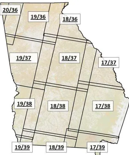
2.1 Study area The study area for this research is the state of Georgia, USA (Fig. 1). As a whole, Geor-gia is a typical southern state with 66.7% of forest cover. It has over 9.7 million hectares of forestland, of which approximately 45% are conifer, 42% are deciduous, 12% are a mixed forest type, and the remaining percentage non-stocked (Cieszewski and Lowe 2007). Adding to the complexity of the landscape, an approximate 650,000 non-industrial landowners hold 75% of the forestland whose average parcel size is decreasing (Georgia Forestry Commission, 2008).
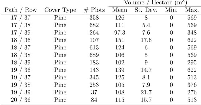
There are distinct differences in the composition of Georgia forests when comparing its locations from north to south. Hardwood ecosystems dominate the areas in the north part of Georgia (Fig. 2A) (Tab.1). The forests transition to conifer-dominated ecosystems as one proceeds southward and to the east (Fig. 2B) (Tab. 1).
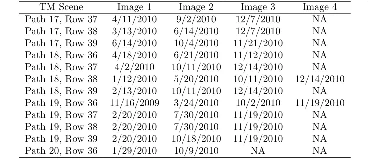
2.2 Satellite imagery We used Landsat 5 Thematic Mapper satellite imagery to model the cubic-meter per hectare estimates using the k nearest neighbor approach. We attempted to attain imagery from the leaf-off season early in the year, leaf-on from the summer months, and another leaf-off image from late in the year. However, this was not possible in all cases (Tab. 2) due to cloudy conditions. We acquired two to four cloud-free images for each of the 12 scenes that wholly or partially cover most of the state. A minimum of eight well-distributed ground control points were located on each scene and the root-mean square error calculated using the early leaf-off scene as the base image. No RMSE exceeded 30 meters. A visual inspection revealed no egregious misalignment in the imagery. Two UTM zones, zone 16 and zone 17,
Figure 1: The 12 Landsat WRS 2 scenes included in the study.
Figure 2: Total volume summarized by FIA regions for the A) coniferous forestland, and B) deciduous forest-land for the state of Georgia.
overlap the state. To facilitate processing, we created a custom coordinate system definition that shifted UTM zone 17 west by 500,000 meters and projected each image to this custom UTM zone. Landsat 5 Thematic Mapper bands 1 – 5 and 7 from each image were composited and used at the 30 meter resolution.
Table 1: Forestland area and total volume summarized by FIA regions reported by the FIA.
Conifer Forest Mixed Forest Deciduous Forest FIA Region Forestland Volume Forestland Volume Forestland Volume
(1000 ha) (Mil. m3) (1000 ha) (Mil. m3) (1000 ha) (Mil. m3)
Northern 228.2 486.4 189 435 782.3 1,781.00
North Central 452.4 911.4 176 314.8 679.5 1,504.20 Central 1,487.20 2,378.30 340.7 463 1,241.20 2,060.70 Southeastern 1,764.80 2,560.40 311.6 392.5 1,109.60 1,678.20 Southwestern 568.2 836.9 145.7 182.9 446.4 695.7
Table 2: Acquisition dates of the Landsat 5 satellite imagery used in the volume estimation processes. TM Scene Image 1 Image 2 Image 3 Image 4
Path 17, Row 37 4/11/2010 9/2/2010 12/7/2010 NA Path 17, Row 38 3/13/2010 6/14/2010 12/7/2010 NA Path 17, Row 39 6/14/2010 10/4/2010 11/21/2010 NA Path 18, Row 36 4/18/2010 6/21/2010 11/12/2010 NA Path 18, Row 37 4/2/2010 10/11/2010 12/14/2010 NA Path 18, Row 38 1/12/2010 5/20/2010 10/11/2010 12/14/2010 Path 18, Row 39 2/13/2010 10/11/2010 12/14/2010 NA Path 19, Row 36 11/16/2009 3/24/2010 10/2/2010 11/19/2010 Path 19, Row 37 2/20/2010 7/30/2010 11/19/2010 NA Path 19, Row 38 2/20/2010 7/30/2010 11/19/2010 NA Path 19, Row 39 2/20/2010 10/18/2010 11/19/2010 NA Path 20, Row 36 1/29/2010 10/9/2010 NA NA
imagery using their field measured GPS locations at the Southern Research Station in Knoxville, Tennessee in December of 2010. We used a series of arcpy (ESRI 2010) scripts to extract the TM band 1 – 5 and 7 pixel values for each FIA cruise locations for all images used in this study (Tab. 2).
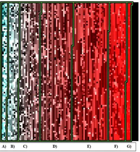
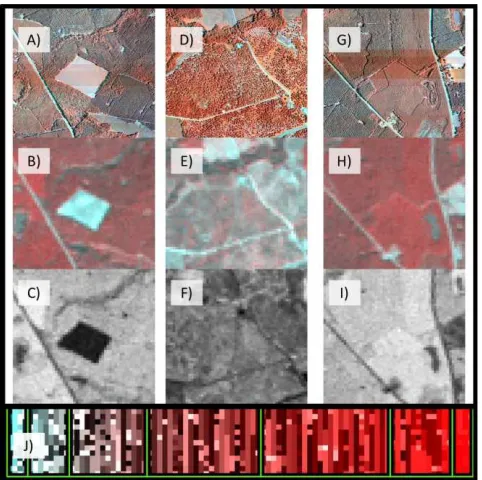
A fundamental aspect of the FIA’s measurement pro-tocol is the fact that measured plots shall not be given preferential treatment by the inventory crew or the pub-lic. The landowner is permitted to manage the forest as they see fit. Thus, there is the possibility that the database may contain outdated information about a plot since any changes to the land that occurs after the in-ventory are not recorded until the next measurement cy-cle. Absent of the plot locations outside the FIA’s data center, we were unable to perform a visual inspection of the TM data at each plot center. However, we did evaluate the spectral information stored in the training sample list using a series of pseudo-image composites, where the ”pseudo-image composites” refer to an image whose pixels have been sequentially rearranged from the lowest NDVI (Eq. 1) (on the left) to the highest NDVI (on the right). We used the following steps to generate the pseudo-images for each scene:
1. sort the training samples according to their NDVI
(Eq. 1) values,
2. reorganize the data into a grid that stores the in-formation from one TM band,
3. repeat step 2 for each spectral band in the training sample list,
4. import each band into ArcGIS, and generate the pseudo-image using the Composite Bands com-mand, and then
5. repeat steps 2 and 4 for the NDVI values.
N DV I= N IR−RED
N IR+RED (1)
where: NIR is the near-infrared layer (TM band 4), and RED is the red layer (TM band 3).
represented in sections A – G as seen in Figure 4. The pixels in sections A) and B) were captured in areas void of green vegetation such as a cultivated field (Fig. 4) or a place inundated with water. Near the other end of the NDVI spectrum, the samples in frame F) (Fig. 3) are sites captured in mature forested areas with full canopy closure (Fig. 4). The sites in frames C through E con-tain samples from old fields, young pine plantations, and thinned forests. Frame G contained the samples with the highest NDVI values. These are cropland sites with abundant, low-lying, fast green vegetation. We used the forested/non-forested thresholds determined by this pro-cess for each scene to assess which, if any, FIA plots had been harvested between the time a plot was measured and the capture of the late-winter TM image. We as-signed those plots a volume per hectare (m3) equal to zero.
We used the Forest Vegetation Simulator (Wykoff et al. 1986, Dixon 2002) to project the FIA field measurements to a common end-of-year 2010. These data are our 2010 common timeline FIA data. We implemented the SN variant and accepted the data processing defaults. The projected dataset contains 6,367 total plots that we have classified as deciduous, mixed, or evergreen according to their dominant specie representation (Tab. 3). There were 150 non-stocked and 2,122 non-forested plots within the state that were not used in the analysis.
We stratified the plots further by the WRS2 scene boundaries (Fig. 1). There is overlap among the scenes in both a north-south and east-west direction so some plots were used multiple times in different scene-level calculations (Tab. 4). These stratified data are the source of the target mean used in the scene-level scal-ing process and as the input training samples used in the volume estimation process. The data files, one for each TM scene, includes FIA plot age, cubic-meter basal area per hectare (BA), cubic-meter volume per hectare (CF), county FIPS code, the TM scene identifier, and the TM spectral summaries that were recorded at each plot center.
We obtained 918 conifer forest polygons and associ-ated stand summary information from our various in-dustrial partners with holdings in WRS2 path 18, row 37. We visually inspected each area on the early and late in the year leaf-off TM and on the 2010 USDA Farm Service Agency National Agriculture Imagery Program aerial photography to ensure the data did not include any partially harvested stands. We manually recoded the stand summaries to zero for any stand that reflected a total harvest. We projected the individual stand ages, volumes and basal area measures to a common 2010 end-of-year timeline. The final industrial data set contained 19,210 hectares. Their ages ranged from zero to 61 and
Figure 3: Pseudo-Landsat image generated from FIA sample sites representing A) bare ground sites, B-C) the transition to forest, D-F) the transition to a closed canopy forest, and G) cropland.
average volume per hectare was 158 m3.
2.4 Land cover We used a composited 2008 Land Use Trends Land Cover of Georgia (GLUT) (NARSAL 2006) and National Land Cover Data (NLCD) 2006 (US-DOI, 2006) to stratify the land base into generic conifer, mixed forest, and deciduous forest types. The composite was created using a raster intersection where
Composite Land Cover=GLUT∗1000 +NLCD.
Table 3: Summary of age, basal area, and cubic-meter volume per hectare for all FIA ground measurements. Hardwood Mix Pine Non-stocked No Forest
# of Stands 1,628 634 1,833 150 2,122
Age Mean 48 38 27 3 0
St. Dev. 30 24 17 2 0
Min. 0 1 0 0 0
Max. 149 162 115 5 0
Basal Area (m2) Mean 9.1 21.8 21.8 0 0
St. Dev. 4.9 10.3 10.6 0 0
Min. 0 0 0 0 0
Max. 38.3 60.4 98.7 0 0
Vol / Ha (m3) Mean 144.1 125 117 0 0
St. Dev. 109.8 89.8 83.2 0 0
Min. 0 0 0 0 0
Max. 810.6 436 622 0 0
Table 4: Summary of 2010 common timeline FIA plot measurements for the 12 TM scenes encompassing the state of Georgia.
Volume / Hectare (m3) Path / Row Cover Type # Plots Mean St. Dev. Min. Max.
17 / 37 Pine 358 126 8 0 569
17 / 38 Pine 682 111 5.4 0 569
17 / 39 Pine 264 97.3 7.6 0 348
18 / 36 Pine 107 151 17.6 0 622
18 / 37 Pine 613 124 6 0 569
18 / 38 Pine 689 106 5 0 569
18 / 39 Pine 183 102 9 0 295
19 / 36 Pine 143 139 14.7 0 622
19 / 37 Pine 345 125 8.1 0 513
19 / 38 Pine 253 105 7.9 0 376
19 / 39 Pine 37 108 21.7 0 276
20 / 36 Pine 84 115 15.7 0 513
dataset. Adhering to the above re-classification scheme, we labeled 44% of stands as conifer, 18% as mixed, and 37% as deciduous class.
2.5 Software We used a variety of commercial soft-ware and in-house programs to process the data. Im-age co-registration, data projection, land cover re-classification, and data cataloging tasks were performed in ESRI’s ArcGIS (ESRI 2010) and ERDAS’ Imagine (ERDAS 2010). We converted the data layers among common GIS image formats and generic binary formats using the GDAL interfaced with Python (Van Rossum 2003) and Perl (The Perl Foundation). We developed custom programs written with Lahey/Fujitsu LF95 v. 8.1b Fortran compiler to implement the nearest-neighbor processing, data summarization, and image generation.
2.6 Initial KNN estimation based on the FIA data In this study, the volume prediction for a pixel
was determined using:
ˆ
yi= 1
k
k X
j=1
yji
where ˆyi is the predicted value for pixel i; and{yij, j= 1,2, ..., k} are the k−spectrally nearest response values stored in the training list.
Figure 4: Visually assessed A-C) non-forest, D-F) sparse forest, and G-I) closed canopy sites as they relate to samples in the J) pseudo-Landsat image (Figure 3 and how they appear in the 2010 color-infrared NAIP (A, D, G), the winter TM (B, E, H), and the NDVI (C, F, I) images.
(2002), the optimal K was selected as the value of k that produces an RMSE (Eq. 2) no larger than 2.5% of the minimum (RMSE value across the same range of K).
RM SE= s
P6
i=1(yi−yˆi)2
n (2)
where yi is the ground-observed, assumed to be true, measurement for samplei, ˆyi is the predicted value for samplei, andnis the total number of samples.
It should be noted that the goal in optimal selection of K is not only improving accuracy, but often it is also preserving the co-variance between different predicted variables while preserving the range of their predicted values. The process of generating volume per hectare (m3) estimates for pixel i initiated with the selection of the K-nearest entries in the training list. Nearness in this study refers to the Euclidean spectral distance (ESD) and is calculated using equation 3. The process was executed with the following steps:
1. calculate ESD from each forested pixel i to each entry in the training list having the same composite land cover type,
2. use Fortran’s intrinsic minval and minloc to find the first closest neighbor in the list,
3. store the volume per hectare value associated with the spectrally nearest entry in the training list and mask it from the list of spectral distances,
4. repeat 2 & 3 K times, and then
5. average those samples to form the KNN-based vol-ume per hectare (m3) estimate .
ESD=
v u u t
6 X
i=1
(ji−ki)2 (3)
where ji is the band i value for the jth entry in the training list and ki is the band i value for the current pixel in the image.
An advantage of the KNN method is the ability to make many estimates for a single location given the in-formation available in the training list. The additional information we stored for each pixel included mean spec-tral distance and a blended land cover. The blended land cover was created by storing the majority composite land cover type. We assigned a mixed type where there was no majority.
Table 5: Reclassification matrix used to combine the GLUT and NLCD land cover products. 2008 GLUT
Clear- Decid- Ever- Forested Nonforest NLCD 2006 cut(31) uous(41) green(42) Mixed(43) Wetland(91) Wet.(93) Deciduous(41) Ever. Decid. Mixed Mixed Decid. NA Evergreen (42) Ever. Mixed Ever. Mixed Ever. NA
Mixed (43) Ever. Mixed Mixed Mixed Mixed NA
Evergreen (52) Ever. Mixed Ever. Mixed Ever. NA Clearcut (71) Ever. Decid. Ever. Mixed Ever. NA
Crop (81, 82) Ever. Decid. Ever. Mixed NA NA
Wetland (90) Ever. Decid. Ever. Mixed Decid. Decid.
2.7 Mean-balancing to the FIA mean volume per-hectare The objective of the Mean Balancing pro-cess is to remove any potential bias in the estimated mean by adjusting individual pixel estimates up or down so the TM-based mean for an area, in this study a Land-sat scene, equals the mean of the FIA plot measurements from the same area. We implemented two balancing methods. Scaling in the first method, we refer to it in this paper asordered Mean Balancing, is based on each pixel’s Euclidean spectral distance where those cells with large ESD values are adjusted more often. Throughout the iterative process, pixels with the largest Euclidean spectral distance are adjusted first. In each subsequent pass, the ESD threshold for pixel selection and adjust-ment is lowered to include a larger number of pixels. Some pixels, especially those with a large ESD, may be adjusted multiple times while it is possible others are not adjusted at all. Each TM scene was processed sep-arately as were the conifer, mixed, and deciduous cover types as denoted in LCOV dataset. The protocol we followed is as follows:
1. calculate the TM-based mean volume per hectare (VACL) for a TM scene, include only cells at-tributed with the current LCOV type (conifer, de-ciduous, or mixed);
2. calculate the mean volume per hectare of the FIA plots (VACF) that fall within the same TM scene and are attributed with the current LCOV type (conifer, deciduous, or mixed);
3. select the pixels equal to or larger than the ESD threshold, and either
(a) adjust the selected pixels by the ratio of the maximum FIA plot volume per hectare to the maximum estimated volume per hectare repre-sented in this set of pixels if VACL is less than VACF, or
(b) decrease the selected pixel values by 2.5% if VACL is greater than VACF;
4. recalculate VACL,
5. repeat steps 3 and 4 until VACL is within 2% of VACF, and then
6. rescale all pixels by the ratio of VACF to VACL to ensure the balanced mean volume per hectare pixel estimates for area equals the FIA’s estimate from the same area.
In the second method, pixel values were scaled propor-tionally by the ratio of the FIA target mean, VACF, to the TM-based mean volume per hectare, VACL. In this paper, we refer to this approach as proportional Mean Balancing.
2.8 Fusion of industry and initial KNN esti-mates We demonstrate an additional improvement to our spatially explicit inventory with the fusion of in-formation from a high-intensity ground-based inventory of industrial pine sites in the central Georgia, path 18, row 37 scene. The goal of this process was to incorpo-rate those measurements we think are highly accuincorpo-rate into our TM-based volume estimates and preserve them throughout the balancing process. Equalization was im-plemented on a stand-by-stand basis where only the pix-els within an inventoried stand were adjusted. Pixel es-timates for areas outside these managed areas were not modified. For each stand individually, we:
1. determined the mean of the initial KNN estimate for a given stand, then
2. adjusted the initial KNN estimates within its stand boundary by the ratio of industry and KNN means, and
3. reset the ESD measure for each of the pixels within the given stand boundary to zero (indicating a very accurate estimate) and then
By resetting the ESD measures within each stand to zero, we reduce the likelihood, but do not eliminate the possibility; an individual estimate will be adjusted dur-ing the Mean Balancdur-ing process.
Assessment
We present the leave-one-out RMSE associated with each optimal K (Fig. 5) as a measure of accuracy of the initial KNN estimation process. Additionally, we calculated mean absolute errors (MAE) (Eq. 4) for the Mean Balancing results. We also present summaries of the Mean Balancing processes for each scene for the pine type contained in LCOV for the initial KNN estimates and the Mean Balanced estimates.
M AE = Pn
i=1|ˆyi−yi|
n (4)
where yi is the ground-observed, assumed to be true, measurement for samplei, ˆyi is the predicted value for samplei; andnis the total number of samples.
We present an assessment of the estimates generated by the 1) initial KNN, 2) the two Mean Balancing ap-proaches, and the 3) industry-infused and Mean Bal-anced processes for the central-Georgia scene, path 18, row 37. The field measurements and GIS data obtained from our industrial partners were not used in the first two estimation routines. Therefore, we use the RMSE and MAE calculated across each industrial stand as an assessment of their accuracy based on an independent, albeit limited in terms of forest type, data source. The industrial data is an integral part of the industry-fused process, so we do not consider them suitable samples for independent validation. However, we present their sum-maries to confirm the improvement in prediction accu-racy achieved through this process.
Finally, to demonstrate the varying results one would attain by querying the 1) standard FIA database, the 2) initial KNN, both 3) Mean Balanced, and the 4) industry-infused data. We present the results of a series of queries at varying scales. We first present summaries for Hancock County, Georgia for the conifer type. There are 97 industrial stands, approximately 2,023 hectares, located in the county. The final two summaries are cen-tered at 33.3141 degrees north and 82.9368 west with a radius of1/2mile (203.4 hectares) and 3.5 miles (9,967.1 hectares). There are five industry stands within the 3.5-mile radius that encompass 83 hectares and one stand less than 8.1 hectares in size within the 0.5-mile radius.
3
Results
The path 19, row 39 scene is located in the extreme southwestern part of the state. The image covers ap-proximately 74,866.9 hectares of forested land and con-tains 69 FIA plots. The scene with the next smallest
coverage of the state, path 18, row 39, encompasses 1.2 million hectares of forested land and 339 forested FIA plots. Due to the small number of plots and a relatively large percentage of overlap by adjacent scenes, nearly 88%, we processed the path 19, row 39 data using K=1. While we scaled the volume per hectare estimates to its FIA scene mean using the same approach as the other scenes, we used the estimates from the adjacent scenes in the overlapping areas (path 19, row 38 and path 18, row 39) when possible. Unless specified, the following sections focus on the remaining 11 scenes used in this study.
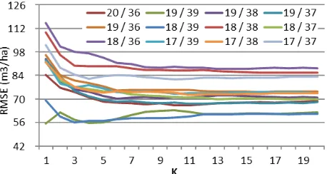
Figure 5: Root-mean squared error measures for K=1 to K=20 for the 12 TM scenes that were generated during the determination of the optimal K
3.1 Selection of the optimal K The leave-one-out KNN assessment of cubic-meter volume per hectare based on the training data revealed an initial decrease in RMSE as the number of neighbors was increased. The gain in accuracy continued from K=3 to K=10 and then leveled off (Fig. 5, Tab. 6). Root-mean squared error values for the optimal K ranged from 55.3 m3/ha 55% of the FIA mean for path 19, row 39, to 87.2 m3/ha, or 71% of the FIA mean for path 18, row 38 (Tab. 6).
The compression of the range of initial volume per hectare estimates is apparent in this study. Initial vol-ume per hectare estimates assessed on the entries of the training list data ranged from 0 to 388.6 m3/ha, less than half of the range of the FIA measurements (Fig. 6). The KNN-derived mean for the training list entries was 21% below the mean calculated from the FIA data, 101.7 m3/ha and 129.5 m3/ha, respectively.
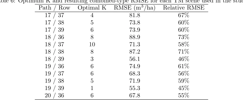
Table 6: Optimum K and resulting combined-type RMSE for each TM scene used in the study. Path / Row Optimal K RMSE (m3/ha) Relative RMSE
17 / 37 4 81.8 67%
17 / 38 5 73.8 60%
17 / 39 6 73.9 60%
18 / 36 8 88.9 73%
18 / 37 10 71.3 58%
18 / 38 8 87.2 71%
18 / 39 3 56.1 46%
19 / 36 6 74.9 61%
19 / 37 6 68.3 56%
19 / 38 5 71.9 59%
19 / 39 1 55.3 45%
20 / 36 6 67.8 55%
LCOV, 4.6 million hectares of deciduous, and 2.9 million hectares of mixed forest type.
3.2 Model assessment The summaries shown below are products of an assessment made simultaneously on the training list samples compiled during the estimation processes where the training list entries were treated as a separate list of pixels in need of an estimate. The cover type designations used in these summaries were assigned by the LCOV data layer.
Initial KNN point estimates of conifer volume per hectare (m3), were on average 22% below the 2010 com-mon timeline FIA estimates (Tab. 7), the ordered Mean Balanced estimates 13% below the 2010 common time-line FIA estimates, and the proportional Mean Balanced estimates were, on average, 26% above the 2010 com-mon timeline FIA estimates. Minimum RMSE for the initial KNN, 69.9 m3/ha, and both the ordered and pro-portional Mean balanced processes, 72 m3/ha and 56.3 m3/ha, respectively, occurred in the southern Georgia 18/39 scene. However, the maximum RMSE occurred in different scenes for each model. The maximum RMSE and MAE for the initial KNN process occurred in the south-central Georgia scene 18/38, 101.3 m3/ha; the ex-treme northwestern Georgia scene 20/36 for the ordered Mean Balancing approach, 129.9 m3/ha, and in the ex-treme north-central Georgia scene 19/36 for the propor-tional Mean Balancing approach, 45.9 m3/ha.
The greatest differences between the initial KNN and both Mean Balanced processes occurred in the treme north-central Georgia scene 19/36 and the ex-treme northwestern Georgia 20/36 scene. The ordered Mean Balancing procedure increased the mean estimate, assessed at each FIA sample point, by 86%, and by more than 209% for the proportional Mean Balancing pro-cess. The smallest difference between the initial KNN and both Mean Balancing process occurred in the
cen-Figure 6: Histogram comparing the distributions of the FIA and the remotely sensed estimates made during the initial KNN process.
tral Georgia scene 18/37 with a difference of less than 2% for ordered Mean Balancing and by less than 38% for the proportional Mean Balancing process (Tab. 7).
3.3 Scene-wide summaries Summaries of the en-tire initial KNN and Mean Balanced estimated surfaces follow. All forested pixels are included in these re-sults. The cover type specifications were assigned by the LCOV data layer.
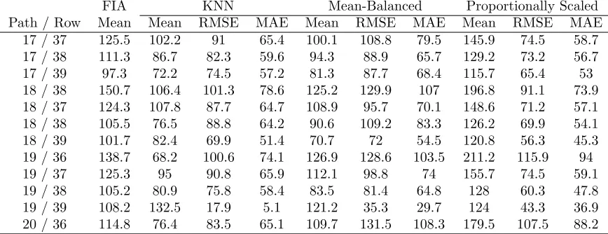
Table 7: Comparison of mean volume estimates (m3/ha), RMSE (m3/ha), and MAE (m3/ha) for training list entries for the: i) conifer Forest Inventory and Analysis (FIA) plot measurements; ii) KNN initial estimates; iii) ordered Mean-Balanced estimates; and iv) proportional Mean-Balanced estimates. (MAE is mean-absolute error).
FIA KNN Mean-Balanced Proportionally Scaled
Path / Row Mean Mean RMSE MAE Mean RMSE MAE Mean RMSE MAE 17 / 37 125.5 102.2 91 65.4 100.1 108.8 79.5 145.9 74.5 58.7 17 / 38 111.3 86.7 82.3 59.6 94.3 88.9 65.7 129.2 73.2 56.7 17 / 39 97.3 72.2 74.5 57.2 81.3 87.7 68.4 115.7 65.4 53 18 / 38 150.7 106.4 101.3 78.6 125.2 129.9 107 196.8 91.1 73.9 18 / 37 124.3 107.8 87.7 64.7 108.9 95.7 70.1 148.6 71.2 57.1 18 / 38 105.5 76.5 88.8 64.2 90.6 109.2 83.3 126.2 69.9 54.1 18 / 39 101.7 82.4 69.9 51.4 70.7 72 54.5 120.8 56.3 45.3 19 / 36 138.7 68.2 100.6 74.1 126.9 128.6 103.5 211.2 115.9 94 19 / 37 125.3 95 90.8 65.9 112.1 98.8 74 155.7 74.5 59.1 19 / 38 105.2 80.9 75.8 58.4 83.5 81.4 64.8 128 60.3 47.8 19 / 39 108.2 132.5 17.9 5.1 121.2 35.3 29.7 124 43.3 36.9 20 / 36 114.8 76.4 83.5 65.1 109.7 131.5 108.3 179.5 107.5 88.2
Balancing process yielding a range of volumes from 0 m3/ha to 808 m3/ha (Tab. 9)
The initial conifer mean in the northern scene, path 19, row 36, was 34% below the FIA target (Tab. 8). In order to raise that scene’s conifer mean to the appropri-ate level, 100% of the conifer pixels (375,378 hectares) had to be adjusted during the ordered Mean Balanc-ing processes. This resulted in the range of data beBalanc-ing increased from 0-395.6 m3/ha to 0-795.3 m3/ha with a mean of 1,983 m3/ha, which is equal to the FIA’s. One-hundred percent of the data were adjusted during the proportional Mean Balancing process which yielded the target mean of 138.8 m3/ha and a similar range of es-timates from 0 to 808 m3/ha (Tab. 9). However, the standard deviation was more than twice as large as those from the ordered mean Balancing process, 116.6 m3/ha and 50.2 m3/ha, respectively.
3.4 Fusion of industrial data in path 18, row 37
The path 18, row 37 mean of the initial KNN-based es-timates for conifer volume per hectare were more than 12% below the 2010 common timeline FIA estimate (Tab. 8). After scaling, the scene-wide conifer means were all near equal to the 18/38 FIA Target (+/- 0.2%). The maximum conifer pixel estimate for the ordered Mean Balanced and Industry Fused routines were both almost twice its FIA and initial KNN counterparts and the maximum value yielded from the proportional Mean Balance routine was 15% larger (Tab. 10).
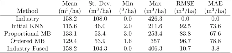
The mean stand volume per hectare produced by the initial KNN estimation routine was 27% below the mean calculated from the industry ground measure-ments (Tab. 11) and the range of predicted stand means was half. The ordered Mean Balancing process
aver-age was 18% below the industry’s measure with a com-pressed range of estimates of almost 17% and the pro-portional Mean Balancing mean 16% lower with a com-pressed range of almost half. By design, the average stand cubic foot volume per hectare and the industry measures are nearly equal. While the means are equal, the range of individual pixel estimates is 10% lower. The initial KNN and the ordered Mean Balancing pro-cess yielded similar RMSE measures of 92.5 m3/ha and 96.7 m3/ha, and MAE measures of 73.6 m3/ha and 78.8 m3/ha, respectively (Tab. 11), only slightly higher than those from the proportional Mean Balanced data. The RMSE and MAE from the industry-fused process was nearly 60% lower, 10.7 m3/ha and 3.8 m3/ha, respec-tively.
The scatter plots in Figure 7 reveal the weak positive relationship between the industry observed stand’s cu-bic foot volume and its remotely sensed estimates using the initial KNN procedure (Fig. 7A), the proportional Mean Balancing (Fig. 7B), the Mean Balancing routine (Fig. 7C). Purposely through the scaling of individual estimates within each industry stand, there is a strong positive relationship with the industry measures and the industry-fused estimates (Fig. 7D). The effects of the scaling that occurred during the Mean Balancing pro-cess (Fig. 7C) are apparent throughout the extent of the industry measurements. The range of estimates for the zero-volume samples (i.e. harvested sites) expanded from 0 to just above 139.9 m3/ha (Fig. 7A) to 0 to approximately 279.9 m3/ha (Fig. 7C).
Table 8: Area of conifer forestland adjusted on the pixel level during the ordered Mean Balancing processes. Initial Mean Adjusted Area Adjusted Area Adjusted Mean Max. Est. Path / Row (% of FIA Mean) (ha) (%) (St. Dev.)(m3/ha) (m3/ha)
17 / 37 -13% 7,481.40 2% 125.5 (68.6) 637
17 / 38 -20% 78,690.80 6% 111.3 ( 66.1) 625
17 / 39 -23% 62,303.40 12% 97.3 (50.1) 381
18 / 36 -32% 162,672.80 100% 150.7 (66.0) 472
18 / 37 -12% 42,196.60 4% 124.3 (67.7) 606
18 / 38 -27% 1,182,838.10 100% 105.4 (66.9) 244
18 / 39 -39% 33,265.60 12% 101.7 (50.2) 300
19 / 36 0.34 375,378.60 100% 138.8 (50.2) 795
19 / 37 30% 132,418.10 20% 125.4 (82.8) 570
19 / 38 -23% 54,152.70 12% 105.2 (60.6) 414
19 / 39 -2% 6.5 ¡1% 108.2 (59.9) 279
20 / 36 -49% 172,600.60 100% 114.8 (82.6) 273
Table 9: Area of conifer forestland adjusted on the pixel level during the proportional Mean Balancing processes. Initial Mean Adjusted Area Adjusted Area Adjusted Mean Max. Est. Path / Row (% of FIA Mean) (ha) (%) (St. Dev.)(m3/ha) (m3/ha)
17 / 37 -13% 463,276 100% 125.5 (68.6) 426
17 / 38 -20% 1,394,528 100% 111.3 ( 66.1) 439
17 / 39 -23% 491,604 100% 97.3 (50.1) 330
18 / 36 -32% 158,057 100% 150.7 (66.0) 473
18 / 37 -12% 1,032,216 100% 124.3 (67.7) 360
18 / 38 -27% 1,132,081 100% 105.4 (66.9) 407
18 / 39 -39% 258,125 100% 101.7 (50.2) 290
19 / 36 -34% 339,060 100% 138.8 (50.2) 808
19 / 37 -30% 644,264 100% 125.4 (82.8) 490
19 / 38 -23% 434,758 100% 105.2 (60.6) 347
19 / 39 -2% 43,342 100% 108.2 (59.9) 280
20 / 36 -49% 146,237 100% 114.8 (82.6) 453
Table 10: Conifer volume per hectare estimates from the 2010 common timeline FIA and generated from the four remote sensing methods for the path 18, row 37 scene.
Method MEAN (m3/ha) St. Dev. (m3/ha) Max (m3/ha)
2010 Common Timeline FIA 124 6 311
Initial KNN 110 60 311
Proportional MB 124 67 360
Ordered MB 124 68 606
Industry Fused 124 83 541
Table 11: Path 18, row 37 stand-level comparison of mean conifer volume per hectare generated from the four estimates based on remote sensing.
Mean St. Dev. Min Max RMSE MAE
Method (m3/ha) (m3/ha) (3/ha) (m3/ha) (m3/ha) (m3/ha)
Industry 158.2 108.0 0.0 426.3 0.0 0.0
Initial KNN 115.6 46.0 2.0 211.6 92.5 73.6 Proportional MB 133.1 53.4 3.0 253.4 83.8 67.6
Ordered MB 129.4 53.9 1.6 357 96.7 78.8
Figure 7: Scatter plots reflecting the volume per hectare (m3) estimates for each industry stand from the A) ini-tial KNN, the B) proportional Mean Balancing, C) the ordered Mean Balancing, and the D) industry-fused pro-cesses.
12). The FIA reports 56,205 hectares of coniferous forestland while LCOV represents 56,195 total conifer hectares. Each of the remotely sensed processes yielded a mean conifer volume per hectare larger than what the FIA reported. The initial KNN process yields a mean volume per hectare of 125.8 m3/ha, 17% more than the FIA; ordered Mean Balancing estimates 133.5 m3/ha, 25% more, proportional Mean Balancing estimates 143.2 m3/ha, 34% more, and the industry-fused process yields an estimate of 135.3 m3/ha (Tab. 12), 26% more than the FIA. The difference between the FIA’s estimate, 213 million m3 and the remote sensing estimates for total conifer volume ranged from 16% to 25%. The initial KNN process yields 247 million m3, ordered Mean Bal-ancing 262 million m3, proportional Mean Balancing 247 million m3, and the industry-fused process 266 million m3.
The FIA reported 2,269.1 hectares (Tab. 13) of conifer forestland area in the 3.5-mile radius query area. How-ever, the LCOV layer reports 4,468 hectares of conifer-classified pixels. All remotely sensed conifer volume per hectare estimates were lower than the FIA’s reported value. FIA reports a volume per hectare of 259.3 m3 while the TM-derived data reports a volume per hectare of 120.3 to 146.7 m3 (Tab. 13). FIA reports no forest-land area or volume in the half-mile query (Tab. 14). The remotely sensed estimates in this query area ranged from a mean conifer volume per hectare of 142.5 m3from the initial KNN estimate to 163.2 m3 from the propor-tional Mean Balanced data.
4
Discussion
In the study described here we used the novel ap-proach of Mean Balancing for removing bias from KNN estimates based on the FIA data and industrial inven-tory data, modeled on satellite imagery for the purpose of redistributing the FIA pine inventory means to pixel size areas of pine forests. We based the approach on the rationalization for balancing an inventory to an un-biased total presented by Iles (2009). In essence, this approach states that any process resulting in the same total as an unbiased estimate is itself unbiased. The principle usefulness of this approach is fusing the large area FIA information with other data for the purpose of obtaining useful small area estimates while maintaining the statistical integrity of the landscape level inventory. Though Iles (2009) balanced on the total volume re-ported from a large-area timber inventory, we balanced on the means reported by the FIA, which essentially rep-resents the same principle. In this approach, we allowed individual pixel estimates to adjust upward or down-ward until the remote sensing-based mean volume per hectare (m3) equalized with the mean derived from the FIA plot measurements and projected to a 2010 com-mon timeline. We used two methods of balancing of which one was indiscriminate to any variables and con-sisted of equal scaling of all estimated values to achieve the desired mean. The other method was based on scal-ing each estimate proportionally to its pixel’s ESD, thus giving more stability to better predict estimates while scaling more the poorer estimates. In theory the later approach seems more desirable and has strong logical basis; however, in our example it produced less accurate estimates for the testing data. Based on these results we conclude that further research is need in this area to im-prove the discriminate algorithm, because it seems that estimates from better matched stands should be more accurate than estimates from mismatched stands, which would suggest that they should be changed less.
This inventory of Georgia differentiates itself from other large-area, remote sensing-based inventories in the northeastern United States and abroad (McRoberts et al. 2010, Tomppo et al. 2008, McRoberts et al. 2009) in the manner bias is addressed. Recommendations for minimizing bias are the incorpo-ration of a weighting factor during the nearest neigh-bor process (Katila 2006, McRoberts 2009), general-ization or segmentation (Hyvonen et al. 2005, Wood-cock et al. 2001) and the careful selection of the optimal K (McRoberts et al. 2002) and method of estimation (Labrecque et al. 2006). We on the other hand accept the statistical integrity of the FIA’s large-area reports and conform our measurements to them.
Table 12: Conifer volume per hectare estimates generated from the FIA, the initial KNN, Mean Balancing, and the industry-fused methods for Hancock County, Georgia.
Area Min Max Mean St. Dev. Volume Method (ha) (m3/ha) (m3/ha) (m3/ha) (m3/ha) (Mil. M3)
FIA Db (Hancock) 56,205 NA NA 107.3 NA 14.9
Initial KNN 56,196 0.0 289.2 125.8 53.7 17.3 Proportional MB 56,196 0.0 329.9 143.2 61.5 18.9 Ordered MB 56,196 0.1 594.1 133.5 60.2 18.3 Industry-fused 56,196 0.1 590.5 135.3 63.7 18.6
Table 13: Query results from the 3.5-mile radius query to the FIA database, the initial KNN, Mean Balancing, and the industry-fused methods for the conifer type.
Area Min Max Mean St. Dev. Volume Method (ha) (m3/ha) (m3/ha) (m3/ha) (m3/ha) (Mil. M3)
FIA Db Query 2,269 NA NA 259.3 NA 1.5
Initial KNN 4,468 0.1 520 129.4 65.8 1.4
Proportional MB 4,468 0.0 355.3 144.8 63.7 1.6 Ordered MB 4,468 0.0 266.5 120.3 56.7 1.3 Industry-fused 4,468 0.1 538.4 130.2 71.4 1.4
Table 14: Query results from the 0.5-mile radius query to the FIA database, the initial KNN, Mean Balancing, and the industry-fused methods for the conifer type.
Area Min Max Mean St. Dev. Volume
Method (ha) (33/ha) (m3/ha) (m3/ha) (m3/ha) (Thousand M3)
FIA Db Query 0 NA NA 0 NA 0
Initial KNN 121 4.5 253.4 142.5 52.3 42.5
Proportional MB 121 5.1 289.0 163.2 59.3 48.8
Ordered MB 121 6.4 462.4 147.2 55.6 43.9
Industry-fused 121 6.4 538.4 157.6 76.5 47.1
equalization decreased the local accuracy of our stand-level volume per hectare (m3) estimates as seen in figures 7A and 7B. Root-mean squared error decreased by 4% and MAE by 7% (Tab. 10) when compared to the ini-tial KNN estimates. However, at a more suitable sum-mary unit for the FIA, scene-level summaries of mean volume per hectare estimates from the balanced models were near equal. Furthermore, after incorporating the small area forest inventory, our local accuracy increased by nearly 2.5 times, while maintaining large area per hectare conformity with the FIA (Tab. 9).
Several issues requiring further assessment were iden-tified throughout this research. We did not explore bal-ancing to the total volume. Our rationalization for us-ing the mean as the target is the fact that volume per hectare is invariant to total area. Total volume, on the other hand, is a product of forestland area and, un-like volume per hectare, fluctuates as that area changes. However, total volume is the measure the FIA reports, so the issue should be addressed.
Second, there is room for more complete utilization of
the small-area measurements. This study only leveraged the information from our industry partners within their stand boundaries. The high resolution ground informa-tion, however, can be used for estimates across the en-tire scene. For instance, Sivanpillai (2006) used similar high resolution forest measurements in conjunction with remote sensing and multivariate regression to estimate age and density for a site in eastern Texas and Meng (Meng et al. 2009b) used high resolution forest informa-tion and satellite imagery with geostatistical techniques for a large-area forest inventory.
assimilate those seemingly unrelated, yet useful bits of information into our high resolution, spatially explicit inventory for the state of Georgia. The inventory re-tains the FIA’s unbiased nature across large areas for volume per hectare (m3), however, unlike the FIA, our inventory also maintains the local accuracies provided by our forest industry partners.
Acknowledgments
We are grateful to the two anonymous reviewers who provided helpful comments for the earlier version of this manuscript.
References
Blackard, J.A., M.V. Finco, E.H. Helmer, G.R. Holden, M.L. Hoppus, D.M. Jacobs, and R.P. Tymcio. 2008. Mapping US forest biomass using nationwide forest inventory data and moderate resolution information. Remote Sensing of Environment. 112: 1658-1677.
Cieszewski, C.J., K. Iles, R.C. Lowe, and M.J. Zasada. 2005. Proof of concept for an approach to a finer reso-lution inventory. Page 69–74. In McRoberts, R. E., G. A. Reams, P. C. Van Deusen, and W. H. McWilliams. Proceedings of the Fifth Annual Forest Inventory and Analysis Symposium. November 18—20, 2003, New Orleans, LA. Gen. Tech. Rep. WO-69. St. Paul, MN: U.S. Department of Agriculture, Forest Service, North Central Research Station. URLhttp://www.nrs.fs. fed.us/pubs/gtr/gtr_wo069.pdf. Accessed Sep. 30, 2014.
Cieszewski, C.J. and R.C. Lowe. 2008. Generic gapfill-ing method for reconstructions of missgapfill-ing data usgapfill-ing KNN approach on multitemporal scene pairings. Fiber Supply Assessment Technical Report 2008-1. Athens, GA: University of Georgia, Warnell School of Forestry and Natural Resources.
Cieszewski, C.J., and R.C. Lowe. 2007. Biomass In-FORM (Interactive Fast Online Reports & Maps). Available at: URL http://www.growthandyield.
com/maps/InFORMB/GA/state_tmplate.swf.
Ac-cessed Sep. 30, 2014.
Dixon, G.E. 2002. Essential FVS: A user’s guide to the Forest Vegetation Simulator. Fort Collins, CO: USDA-Forest Service, USDA-Forest Management Service Center.
Franco-Lopez, H., A.R. Ek., and M.E. Bauer. 2001. Es-timation and mapping of forest stand density, volume, and cover type using the k-nearest neighbors method. Remote Sensing of Environment. 77: 251-274.
Gjertsen, A.K. 2007. Accuracy of Forest Mapping Based on Landsat TM Data and a kNN-based Method. Re-mote Sensing of Environment. 110: 420-430.
Hyvonen, P., A. Pekkarinen, and S. Tuominen. 2005. Segment-level Stand Inventory for Forest Manage-ment. Scandinavian Journal of Forest Research. 20: 75-84.
Iles, K. 2009. ”Total-Balancing” an inventory: A method for unbiased inventories using highly biased non-sample data at variable scales. Mathematical and Computational Forestry & Natural Resource Sciences (MCFNS). 1: 10-13. URLhttp://mcfns.com/index. php/Journal/article/view/MCFNS.1-10. Accessed Sep. 30, 2014.
ERDAS. 2010. ERDAS Imagine Field Guide. Atlanta, GA: Erdas Inc.
ESRI. 2010. ArcMap 10.0. Redlands, CA: Environmen-tal Systems Resource Institute.
Katila, M. 2006. Correcting Map Errors in Forest Inven-tory Estimates for Small Areas. Forest InvenInven-tory. 40: 225-233.
Labrecque, S., R.A. Fournier, J.E. Luther, and D. Piercey. 2006. A Comparison of Four Methods to Map Biomass from Landsat-TM and Inventory Data in Western Newfoundland. Forest Ecology and Manage-ment. 226: 129-144.
McRoberts, R.E. 2012. Estimating Forest Attribute Pa-rameters for Small Areas Using Nearest Neighbors Techniques. Forest Ecology and Management. 272: 3-12.McRoberts, R., E. Tomppo, and E. Naesset. 2010. Advances and Emerging Issues in National Forest In-ventories. Scandinavian Journal of Forest Research. 25: 368-381.
McRoberts, R.E., W.B. Cohen, E. Naesset, S.V. Stehman, and E.O. Tomppo. 2010. Using remotely sensed data to construct and assess forest attribute maps and related spatial products. Scandinavian Jour-nal of Forest Research 25: 340-367.
McRoberts, R.E. 2009. Diagnostic Tools for Nearest Neighbors Techniques When Used with Satellite Im-agery. Remote Sensing of Environment. 113: 489-499.
McRoberts, R.E., D.G. Wendt, M.D. Nelson, and M.H. Hansen. 2002. Stratified Estimation of Forest Area Using Satellite Imagery, Inventory Data, and the k-Nearest Neighbors Technique. Remote Sensing of En-vironment. 81: 457-468.
Meng, Q., B.E. Borders, C.J. Cieszewski, and M. Mad-den. 2009a. Closest Spectral Fit for Removing Clouds and Cloud Shadows. Photogrammetric Engineering and Remote Sensing. 75: 569-576.
Meng, Q., C.J. Cieszewski, and M. Madden. 2009b. Large Area Forest Inventory Using Landsat ETM+: A Geostatistical Approach. ISPRS Journal of Pho-togrammetry and Remote Sensing. 64: 27-36.
Meng, Q., C.J. Cieszewski, M. Madden, and B.E. Bor-ders. 2007. A linear mixed-effects model of biomass and volume of trees using Landsat ETM+ images. For-est Ecology and Management, 244(1), 93-101.Natural Resources Spatial Analysis Laboratory (NARSAL). 2001. Georgia Land Use Trends (GLUT) project data. Athens, GA: University of Georgia, Institute of Ecol-ogy.
Reese, H., M. Nilsson, T.G. Pahl´en, O. Hagner, S. Joyce, U. Tingel¨of, M. Egberth, and H. Olsson. 2010. Coun-trywide Estimates and Data Satellite Using Inventory Forest Variables Using Satellite Data and Field Data From the National Forest Inventory. AMBIO: A Jour-nal of the Human Environment. 32: 542-548.
Sivanpillai, R., C. Smith, R. Srinivasan, M. Messina, and X. Wu. 2006. Estimation of Managed Loblolly Pine Stand Age and Density with Landsat ETM+ Data. Forest Ecology and Management. 223: 247-254.
Tomppo, E., H. Olsson, G. Stahl, M. Nilsson, O. Hagner, and M. Katila. 2008. Combining National Forest In-ventory Field Plots and Remote Sensing Data for For-est Databases. Remote Sensing of Environment. 112: 1982-1999.
Trotter, C.M., J.R. Dymond, and C.J. Goulding. 1997. Estimation of Timber Volume in a Coniferous Planta-tion Forest Using Landsat TM. InternaPlanta-tional Journal of Remote Sensing. 18: 2209-2223.
Van Deusen, P. 2010. Carbon Sequestration Potential of Forest Land: Management for Products and Bioen-ergy Versus Preservation. Biomass and BioenBioen-ergy. 34: 1687-1694.
Van Rossum, G. 2003. An introduction to Python. F. L. Drake (Ed.). Bristol: Network Theory Ltd.
Walker, W.S., J.M Kellndorfer, E. LaPoint, M. Hoppus, and J. Westfall. 2007. An empirical InSAR-optical fu-sion approach to mapping vegetation canopy height. Remote Sensing of Environment. 109: 482-499.
Wayman, J.P. 2000. Landsat TM-based forest area esti-mation using iterative guided spectral class rejection (Doctoral dissertation, Virginia Polytechnic).
Woodcock, C.E., S.A. Macomber, M. Pax-lenney, and W.B. Cohen. 2001. Monitoring Large Areas for Forest Change Using Landsat: Generalization Across Space, Time and Landsat Sensors. Remote Sensing of Envi-ronment. 78: 194-203.