Time-lapse refraction seismic tomography for the detection of ground ice degradation

(1)

www.the-cryosphere.net/4/243/2010/ doi:10.5194/tc-4-243-2010

The Cryosphere

Time-lapse refraction seismic tomography for the

detection of ground ice degradation

C. Hilbich

Institute for Geography, University of Jena, Germany Institute for Geography, University of Zurich, Switzerland

Received: 22 December 2009 – Published in The Cryosphere Discuss.: 27 January 2010 Revised: 27 May 2010 – Accepted: 28 June 2010 – Published: 16 July 2010

Abstract. The ice content of the subsurface is a major factor controlling the natural hazard potential of permafrost degra-dation in alpine terrain. Monitoring of changes in ice con-tent is therefore similarly important as temperature moni-toring in mountain permafrost. Although electrical resistiv-ity tomography monitoring (ERTM) proved to be a valuable tool for the observation of ice degradation, results are often ambiguous or contaminated by inversion artefacts. In the-ory, the sensitivity of P-wave velocity of seismic waves to phase changes between unfrozen water and ice is similar to the sensitivity of electric resistivity. Provided that the gen-eral conditions (lithology, stratigraphy, state of weathering, pore space) remain unchanged over the observation period, temporal changes in the observed travel times of repeated seismic measurements should indicate changes in the ice and water content within the pores and fractures of the subsur-face material. In this paper, a time-lapse refraction seismic tomography (TLST) approach is applied as an independent method to ERTM at two test sites in the Swiss Alps. The ap-proach was tested and validated based on a) the comparison of time-lapse seismograms and analysis of reproducibility of the seismic signal, b) the analysis of time-lapse travel time curves with respect to shifts in travel times and changes in P-wave velocities, and c) the comparison of inverted tomo-grams including the quantification of velocity changes. Re-sults show a high potential of the TLST approach concern-ing the detection of altered subsurface conditions caused by freezing and thawing processes. For velocity changes on the order of 3000 m/s even an unambiguous identification of sig-nificant ice loss is possible.

Correspondence to: C. Hilbich (chilbich@geo.uzh.ch)

1 Motivation

Monitoring of permafrost in polar and mountainous regions becomes more and more important in the context of ongoing global warming. A key parameter concerning slope stability analyses and permafrost modelling purposes is the ice con-tent of the subsurface and its temporal evolution (Gruber and Haeberli, 2007; Harris et al., 2009). Thermal monitoring in boreholes is a common and widespread method to observe permafrost evolution (e.g. Harris and Isaksen, 2008; PER-MOS, 2009), but does only provide indirect insights into ice content changes. Many geophysical methods are more sen-sitive to changes in water content than to temperature vari-ations, and in particular to phase transitions between frozen and unfrozen water. Fortier et al. (1994) showed that varia-tions of apparent resistivity with time can be used to predict unfrozen water and ice contents of the frozen ground. Re-cent studies on the applicability of electrical resistivity to-mography monitoring (ERTM) proved the high sensitivity of electrical resistivity tomography (ERT) to spatio-temporal changes in the subsurface ice and water contents (Hauck, 2002; Hilbich et al., 2008; Kneisel et al., 2008; Hilbich, 2009).

(2)

permafrost ice and from ca. 2000–6000 m/s for both frozen and unfrozen bedrock (e.g. Hauck and Kneisel, 2008). These large ranges and their wide overlap make a differentiation of stratigraphic details in bedrock and/or below the permafrost table (e.g. in rock glaciers or talus slopes) often difficult. To-gether with the comparatively high measurement and pro-cessing efforts, this may be a reason why refraction seismic surveys are less popular in permafrost research than e.g. ERT or GPR measurements. Nevertheless, numerous studies suc-cessfully applied refraction seismic surveys in permafrost terrain (e.g. R¨othlisberger, 1972; Barsch, 1973; Harris and Cook, 1986; Vonder M¨uhll, 1993; Musil et al., 2002; Hauck et al., 2004; Ikeda, 2006; Hausmann et al., 2007; Maurer and Hauck, 2007). Main advantages of the method, com-pared to ERT surveys, are e.g. the much higher depth resolu-tion (Lanz et al., 1998), the potential to exactly localise sharp layer boundaries, the less challenging coupling of the sensors in blocky terrain, or the applicability in terrain with electri-cally conductive infrastructure contaminating the resistivity signal.

Provided that the general subsurface conditions (lithol-ogy, stratigraphy, state of weathering, pore space) remain unchanged over the observation period, changes in the ice and water content within the pores and fractures of the sub-surface material should similarly or even better be detectable by repeated seismic measurements than for ERT. Despite the ambiguities involved in a qualitative interpretation of layers (due to overlapping velocity ranges of different materials), even comparatively small temporal changes in P-wave veloc-ities may indicate zones with significant ice content changes due to seasonal variations or long-term climate change.

According to the theoretical suitability of repeated seismic measurements to permafrost related research, a time-lapse refraction seismic tomography (TLST) approach and its po-tential to observe temporal changes in ice and water content in alpine permafrost will be evaluated in this paper.

2 Theory and approach

Apart from a vast research related to reflection seismic mon-itoring of deep reservoirs in exploration geophysics (see e.g. Vesnaver et al., 2003; King, 2005), similar efforts to investigate the potential of a time-lapse refraction seismic tomography approach for the observation of shallow targets have not been reported so far.

In exploration geophysics the detection of reservoir changes is preferably done using reflection seismics due to their high resolution potential at larger depths. How-ever, reflection data rarely provide information on the very shallow parts (5–15 m) of unconsolidated sediments, as re-flections are usually overwhelmed by different coincident-arriving waves. They are more affected by scattering effects in highly heterogeneous material with shallow low velocity layers than seismic refractions (Lanz et al., 1998), which is

the typical situation for mountain permafrost sites. Accord-ing to Lanz et al. (1998) and Musil et al. (2002) refraction seismic tomography is therefore more appropriate for explor-ing the upper 50 m of the subsurface.

For deep reservoirs, a first approach in using time-lapse refraction seismics was introduced by Landrø et al. (2004) for the estimation of reservoir velocity changes. It is based on the fact, that a velocity change by only 1% will change the critical angle of refraction and thus the critical offset for refracted waves, i.e. their first appearance at the surface. For oil reservoirs located at depths of>1000 m this change in critical offset amounts to several tens of meters (Landrø et al., 2004), but for shallow targets this would be reduced to a few centimetres to decimetres, making this approach in-appropriate for mountain permafrost evolution. Concerning shallow applications, no operationally applicable time-lapse refraction seismic approach was published so far, neither for permafrost, nor for other fields of interest.

The presence of ice in the pore spaces of sediments can cause large increases in seismic velocity compared to the ve-locity when the interstitial water is unfrozen (Timur, 1968). Since ice is much stiffer than water, the wave speed is a strongly increasing function of the ice-to-water ratio. How-ever, firm rock is much stiffer than either ice or water, there-fore the wave speed is also a decreasing function of the porosity 8 (Zimmerman and King, 1986). In the litera-ture several approaches to calculate the dependence of vp on ice and water content in an ice-liquid-rock matrix have been formulated, an overview is given by Carcione and Se-riani (1998). Even though the different approaches to model a three-phase medium have different limitations (e.g. restric-tion to unconsolidated or consolidated material), all models simply relate the composite densityρof a medium to the re-spective fractions8of water (8w), ice (8i)and solid rock (8s)and their densitiesρw,ρi, andρs:

ρ=8wρw+8iρi+8sρs, (1) provided that 8w+8i+8s =1. Due to this common assumption, all models presented in Carcione and Seriani (1998) show, despite their differences, similar qualitative de-pendencies between ice, water and the rock material and their respective P-wave velocities. According to Hauck et al. (2008), theoretically, Eq. (1) can be extended including also the air-filled pore space to account for all components of a subsurface material. Due to the markedly different veloci-ties of air (330 m/s), water (ca. 1500 m/s) and ice (3500 m/s), accordingly, a transition from ice to water (melting) or ice to air (melting and drainage) would result in pronounced veloc-ity changes.

(3)

The velocity change depends mainly on the porosity and the initial saturation, and is thus more pronounced for unconsol-idated coarse-grained sediments than for consolunconsol-idated rocks (Scott et al., 1990).

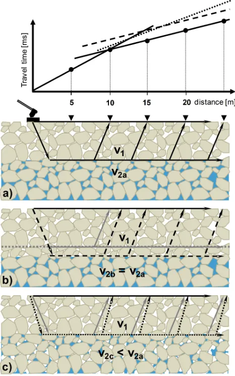
In a qualitative sense, these general dependencies can be used to analyse permafrost evolution via repeated seismic measurements. The principle of a repeated (time-lapse) re-fraction seismic approach is exemplarily illustrated in Fig. 1 for a coarse grained material with water- and/or air filled voids. From a permafrost degradation point of view, not only degradation from above (Fig. 1b) but also an overall warming of the permafrost may be detected by increasing amounts of unfrozen water or air (as a consequence of drain-ing), as roughly indicated in Fig. 1c. Necessary conditions to reliably detect subsurface changes via repeated refraction seismic measurements include constant measurement con-ditions (i.e. source-receiver-geometry and signal generation) between subsequent measurements.

The measured time-lapse seismic data can then be succes-sively processed and analysed using standard methods for tomographic inversion of seismic data. In this study, a re-fraction seismic tomography algorithm is used that recon-structs the 2-D velocity pattern of the subsurface based on an iterative adaptation of synthetic travel times to observed travel times along calculated ray paths of the seismic P-waves (so-called SIRT algorithm, software REFLEXW, Sandmeier, 2008).

A hierarchy of methods has been evaluated to detect tem-poral changes in the subsurface:

(a) The comparison of seismograms from subsequent mea-surement dates (time-lapse seismograms) and analysis of reproducibility of the seismic signal.

(b) The analysis of time-lapse travel time curves with re-spect to resolving possible shifts in travel times and changes in P-wave velocities.

(c) The comparison of inverted tomograms calculated with REFLEXW including the quantification of spatio-temporal velocity changes by calculating the differences between individual tomograms (time-lapse tomogra-phy).

Hereby, the 2-dimensional tomographic approach in (c) was chosen to detect lateral changes in the velocity field. For an exact localisation of vertical discontinuities (if present), a wavefront inversion would give a higher accuracy due to the enhanced smoothing effect in the tomographic approach.

In the following, the potential and limitations for the ap-plication of time-lapse refraction seismic in high mountain permafrost environments will be analysed based on repeated measurements at two sites.

Fig. 1. Idealised principle of time-lapse refraction seismic based

on (a) a two-layer subsurface model with a coarse-blocky unfrozen overburden with air-filled voids and a saturated rock-ice-matrix un-derneath. The lower panels illustrate the change of travel times as a consequence of (b) a vertical shift of the refractor (e.g. the sea-sonally varying interface between frozen and unfrozen conditions), and (c) altered ice (and air) contents within the lower layer causing changes in seismic velocity. The corresponding travel time curves for all three scenarios are given above.

3 Site description and data sets

To evaluate the TLST approach repeated refraction seismic measurements were carried out at two different permafrost test sites in the summer season of 2008. The test sites com-prise a) the ventilated Lapires talus slope in the Valais, and b) the north oriented slope of the Schilthorn summit in the Bernese Alps (see Fig. 2).

(4)

Table 1. Measurement details for the time-lapse refraction seismic test sites (abbreviations: TD = thaw depth, n.a. = notavailable).

Lapires Schilthorn dates of measurement

(respective thaw depths in boreholes)

07/10/2008 (TD 4/2.5 m) 08/18/2008 (TD 5/5 m)

07/11/2008 (TD 1.4/0.2 m) 08/26/2008 (TD 4.5/1.5 m) 08/23/2009 (TD 4.2/n.a.)

number of geophones 23 24 geophone spacing 8 m 2 m profile length 176 m 46 m number of shot points 24 24 off-end shots (distance from

first/last geophone)

4/4 m –/1 m

sample interval 0.125 ms 0.125 ms (2008) 0.25 ms (2009)

record length 192 ms 128 ms

of metamorphic clasts (mainly gneiss) (Vonder M¨uhll et al., 2007). Excavations for the installation of two cable car py-lons in summer 1998 exposed sediments more or less satu-rated with ice (Lambiel, 1999; Delaloye et al., 2001). The frozen zone starts at around 4 m depth and has a maximum thickness of about 20 m. The thermal regime can be de-scribed as temperate (warm) permafrost. According to De-laloye and Lambiel (2005) the existence of permafrost at this site is (at least partly) due to an internal air circulation that contributes to the cooling of the talus slope. Seismic mea-surements were conducted along a permanent ERT profile (described in Hilbich, 2009) in horizontal direction travers-ing a pylon and a borehole. The ERT data acquired in parallel to the TLST measurements will be shown for comparison in Sect. 5.3. A detailed discussion of the ERTM approach and the data can be found in Hilbich (2009).

The Schilthorn massif with the summit at 2970 m altitude represents a bedrock permafrost site and is located close to Mürren at the transition between the Prealps in the north and the principal chain of the Bernese Alps in the southeast. It consists of metamorphic sedimentary rocks dominated by strongly weathered dark limestone schists with a fine-grained debris cover (up to ca. 5 m thick) around the summit area (Imhof et al., 2000; Vonder Mühll et al., 2007). The presence of permafrost was first observed in 1965 during the construc-tion of the summit staconstruc-tion (Imhof et al., 2000) and further proved by three boreholes drilled into the north facing slope approximately 60 m below the ridge to monitor thermal per-mafrost evolution (Harris et al., 2003). The perper-mafrost base was not reached by the 100 m deep boreholes. Permafrost temperatures at Schilthorn are close to 0◦C, and according to the material exposed during drilling, the ice content seems to be very low (personal communication, D. Vonder Mühll). The average maximum active layer thickness is about 5 m. Seismic measurements were conducted along a permanent

ERT profile (described in Hilbich et al., 2008) in horizontal direction within the north facing slope, traversing the bore-holes. As for the Lapires site, corresponding ERT measure-ments will be shown for comparison in Sect. 5.3.

This study is focused on a detailed analysis of data sets acquired in parallel at both sites in July and August 2008. The first measurement date roughly represents the end of the snowmelt season, when the active layer starts thawing, whereas the second date corresponds to an already well de-veloped thawed active layer. Because of its pronounced changes, this seasonal time-span is well suited to evaluate the general applicability of the TLST approach. To account for the potential to detect not only seasonal but also annual differences, a further data set from Schilthorn after one year (August 2009) will be discussed at the end of the paper. At both sites borehole temperatures are available for validation of the geophysical data. Table 1 summarises the details of data acquisition and the respective active layer depths in the nearby boreholes at the dates of measurement.

4 Data acquisition and processing

(5)

Fig. 2. Photographs of the test sites: (a) Lapires talus slope, and (b) the Schilthorn rock slope. The TLST profile lines and the

posi-tions of the boreholes are highlighted.

The seismic signal was generated by a sledge hammer striking a steel plate or firm boulders where available. Signal stacking of minimum 10–20 stacks was necessary to achieve an adequate signal-to-noise ratio. Depending on the overall length of the profiles up to 40 stacks were carried out for the far shots. Shot points were placed at the midpoint between each pair of geophones to guarantee a high spatial resolution for the tomographic inversion (Maurer and Hauck, 2007). Geophone spacing was 8 m at Lapires and 2 m at Schilthorn. Data processing (first arrival picking, travel time analy-sis, tomographic inversion) was done using the software RE-FLEXW (Sandmeier, 2008). The reconstruction of the 2-D velocity pattern of the subsurface is based on the auto-matic iterative adaptation of synthetic travel times (calcu-lated by forward modelling) to observed travel times using the so-called SIRT (Simultaneous Iterative Reconstruction Technique) inversion algorithm (Sandmeier, 2008). A start-ing model has to be defined that consists ideally of a gradi-ent model with increasing velocities with depth reflecting the

gross structure of the study area. The same starting model was applied for all measurements at each site. According to Lanz et al. (1998) a relatively high velocity gradient of 400 m/s per metre for Lapires and 600 m/s per metre for Schilthorn was chosen to ensure sufficient ray coverage. In contrast to the layer concept illustrated in Fig. 1, the tomo-graphic inversion algorithm of REFLEXW is based on div-ing waves, for which a gradient model is more appropriate as a starting model. Starting from this initial model synthetic travel times are calculated by forward modelling, which are then compared to the observed data. The cell size of the grid was 2 m for Lapires and 0.5 m for Schilthorn. After each it-eration the data were slightly smoothed in x-direction (three cells averaged). Based on the travel time residuals the initial model is adapted and synthetic travel times are again cal-culated for the new model. This iterative process stops as soon as distinct stopping criteria are fulfilled, e.g. if the rel-ative change between subsequent iterations is smaller than a predefined value, or a maximum number of iterations is reached. The same settings were used for all inversions. Ve-locity differences were calculated from individually inverted tomograms to analyse the temporal change in P-wave veloc-ities.

5 Results

5.1 Analysis of seismograms 5.1.1 Lapires

Figure 3a exemplarily illustrates a detailed view of an un-filtered part of a selected seismogram with the traces and picked first arrivals for two measurement dates: 10 July (grey) and 18 August 2008 (red). Striking features of this seismogram are a) the very similar waveforms of correspond-ing traces from both dates pointcorrespond-ing to a high reproducibility of the seismic signal for subsequent measurements, and b) the generally earlier arrival times of the waves in July com-pared to those from August with a time shift of about 1–3 ms between the two dates. The absolute pick uncertainty for the Lapires site is estimated to be around 1 ms, and the relative uncertainty (i.e. the accuracy in correlating two phases for subsequent measurements) is between 0.1–0.5 ms, indicating that the observed time shift is significant.

5.1.2 Schilthorn

(6)

Fig. 3. Detailed view of a time-lapse seismogram from (a) Lapires with traces and picked first arrivals from 10 July (grey) and 18 August 2008

(red), and from (b) Schilthorn with traces and picked first arrivals from 11 July (grey) and 26 August 2008 (red). Note the time shifts of the first arrivals for the later date.

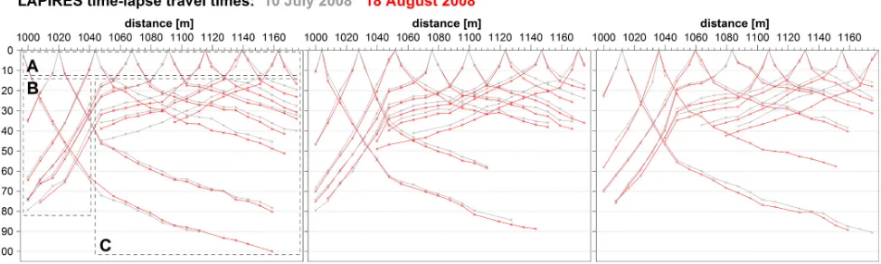
Fig. 4. Comparison of travel times from the Lapires site from 10 July (grey) and 18 August 2008 (red), distributed into three separated plots

for clarity. Zones A, B and C are described in the text. Note, that some unpicked traces may change the slope of the travel time curve.

caused by considerably longer travel paths of the waves due to a lowered refractor depth in August and a correspondingly altered seismic signal, which also prevents an estimation of the relative pick uncertainty between the two data sets. How-ever, first tests on repeated seismic measurements were con-ducted in 2002 at Schilthorn, which yielded very similar data sets for daily measurements and proved the reproducibility of the signal (Schudel, 2003).

5.2 Analysis of travel time curves 5.2.1 Lapires

First arrivals were picked manually for 388 (July) and 484 (August) out of 552 traces for both measurement dates. For data sets from coarse blocky sites with considerable surface roughness the identification of the first arrivals is sometimes complicated by their irregular distribution. In this context the high reproducibility of the signal was therefore utilised to

in-crease the confidence in the identification of the first arrivals by jointly analysing both data sets for first arrival picking (as illustrated in Fig. 3). Especially at far distances from the shot points this “constrained picking” considerably improved the accuracy in identifying the first breaks.

All picked first arrivals are displayed as combined travel time curves in Fig. 4. The superposition of corresponding pairs of travel time curves (grey July, red August) allows the analysis of differences between the two dates (hereby, the complete travel time data set was divided into three different plots for better visibility). The combined travel time curves can provide information on a) changes in the slope of the travel time curves indicating altered ice and water contents of certain layers, and/or b) time shifts in travel times indicating a shift in the depth of a refractor (e.g. the seasonally varying interface between frozen and unfrozen conditions).

(7)

case of small to medium changes in the subsurface. Note, that some unpicked traces for large source-receiver distances cause differences in total travel times for corresponding for-ward and reverse traverses.

Main parts of the travel time curves (indicated in Fig. 4) comprise homogeneously low velocities (400–700 m/s) in the uppermost layer of the whole profile (zone A), only slightly increased velocities (800–1000 m/s) for later arrivals in zone B, and a clear refractor characterised by a sharp ve-locity increase (3000–4500 m/s) in zone C.

Regarding the temporal evolution of travel times, the first arrivals for the data set from July are slightly earlier than for the second measurement in August. Important features of the time-lapse travel time plot are:

(a) small or even absent travel time differences in zones A and B,

(b) significant deviations from the mean displacement for some shots in zone C (e.g. at 1044, 1124, 1172, and 1180 m horizontal distance), which may indicate a change in the form of the refractor (according to Reynolds, 1997), i.e. locally pronounced changes in the refractor depth,

(c) differences between both dates are generally charac-terised by time shifts of the travel time curves rather than by clear changes in the velocities of certain layers. Plotting the travel times against the absolute offset between source and receiver (after Hausmann et al., 2007) reveals a clustering according to the dominant layers of the subsur-face that allows a rough estimation of the mean velocities of the respective materials (indicated in Fig. 5a). As the Lapires site exhibits pronounced lateral differences the com-mon offset plot shows two separate branches with the lower-most branch caused by a delayed arrival (longer travel time) of waves traversing zones B and C instead of only C (up-permost branch). The mean velocity close to the surface is relatively low (ca. 650 m/s) and corresponds to the uncon-solidated coarse blocky layer of the talus slope. Almost no increase in velocity is observed within zone B (mean velocity about 780 m/s), indicating that no clear refractor is detectable within the investigation depth of the survey geometry, thus strongly restricting the information on the left side of the profile. The mean velocity of the only significant refractor observed (zone C) amounts to 3500 m/s and is indicative for ice (R¨othlisberger, 1972).

Figure 5b shows the observed travel time differences be-tween July and August plotted against the absolute source-receiver offset. The majority of travel time differences be-tween August and July are positive indicating an increase in travel time. The dependence of the travel time differences from the shot location is small for all offsets greater 20 m (Fig. 5b), meaning that the travel time shifts are caused close to the surface and only minor velocity changes (correspond-ing to ice content changes) are expected at greater depth.

Fig. 5. (a) Travel times from Lapires for 10 July 2008 (grey)

and 18 August 2008 (red) (as in Fig. 4), here sorted by the ab-solute offset between geophone and shot point (for better visibil-ity of both data sets the x-axis was slightly shifted to the right for 10 July 2008). (b) Travel time differences between August and July, sorted by source-receiver offset.

(8)

Fig. 6. Combined travel time curves for the measurement at Schilthorn from (a) 11 July 2008 (grey) and (b) 26 August 2008 (red). Zones A to D are described in the text.

a basically constant velocity of the surface layer (zone A), and the irregular pattern of the travel times in zone B indicat-ing a pronounced topography of the refractor. Features in the travel time pattern which disappear between July and August (zone C) may be related to ice occurrences, while features consistent over time (zone D) may point to structural infor-mation of the bedrock topography.

A first interpretation of the observed features includes a significant thickening of the low velocity surface layer, i.e. a lowering of the refractor as a consequence of thawing pro-cesses.

The common offset plot of the travel times in Fig. 7a ap-pears very similar for both dates and basically shows two layers with average velocities of about 590 m/s for the sur-face layer and 3500 m/s at greater depth. The velocity of

Fig. 7. Common offset plot of (a) the travel times and (b) the travel

time differences at Schilthorn for 11 July 2008 and 26 August 2008.

the anomalous zone D in Fig. 6 cannot be determined from Fig. 7a. Figure 7b shows the observed travel time differences between July and August 2008 plotted against the absolute source-receiver offset. As for Lapires, the majority of travel time differences are positive denoting an increase in travel time. Again, the dependence of the travel time differences from the shot location is small for all offsets greater 10 m, meaning that the majority of travel time shifts due to veloc-ity changes is caused close to the surface and no pronounced changes are occurring in the deepest part of the profile. 5.3 Analysis of time-lapse tomograms

5.3.1 Lapires

(9)

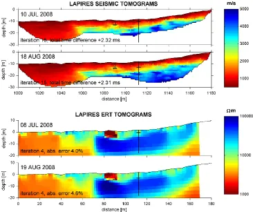
Fig. 8. Comparison of seismic tomograms (upper panels) from 10 July and 18 August 2008 at Lapires with ERT tomograms (lower panels)

from comparable dates. Locations of the pylon and the borehole are indicated, as well as the respective thaw depth at both positions.

As the investigation depth of a refraction seismic survey depends not only on the survey geometry (source-receiver locations) but also on the characteristics of the subsurface layers, the investigation depth at ice-rich permafrost sites is often limited by the presence of a sharp refractor caused by the transition from the unfrozen active layer to the per-mafrost table. The amount of energy reflected/refracted to the surface is a function of the velocity contrast at an inter-face, with high velocity contrasts causing greater fractions of energy to be reflected or refracted to the surface (Burger et al., 2006). By this, the potential to resolve additional refrac-tors at greater depth (e.g. the bedrock interface) decreases substantially. The seismic tomograms in Fig. 8 illustrate this problem: the investigation depth is relatively shallow and does not exceed 15 m on average.

The two tomograms from July and August are largely comparable concerning the overall structure, but exhibit dif-ferent investigation depths and a clear shift in the transi-tion between the low velocity overburden (red colours, cor-responding to zone A in Fig. 4) and the material indicated by blue colours, corresponding to zone C, which is interpreted as the zone containing ice.

To quantitatively analyse the change in P-wave velocities from July to August, the absolute velocity difference (derived

from independent tomographic inversion of both data sets) is displayed in Fig. 9 (upper panel). Note that velocity changes are only shown for the zone resolved by both data sets.

As indicated in Fig. 1, a velocity decrease observed in a time-lapse tomogram (red colours in Fig. 9) may be a con-sequence of either a lowered refractor depth (with basically unchanged layer velocities), or a decrease in layer velocity (with unchanged refractor depth), or a combination of both. To avoid ambiguities in the interpretation, time-lapse tomo-grams must therefore always be evaluated with respect to the absolute velocities in the refraction seismic tomograms (Fig. 8). Here, the information from the seismic tomograms in Fig. 8 corresponds to the observations made from the anal-ysis of travel time differences and indicates that the red zones in Fig. 9 represent a significant downward shift of the refrac-tor, i.e. the advance of the thawing front to greater depth, rather than a significant change of the overall layer veloci-ties.

(10)

Fig. 9. Comparison of temporal change in seismic velocities with resistivity changes. Locations of the pylon and the borehole are indicated,

as well as the respective thaw depths for both dates.

The results of tomographic inversion of the Schilthorn data sets are shown in Fig. 10 (upper panels) together with the corresponding ERT tomograms from the same date (lower panels, which will be interpreted together with the TLST re-sults in Sect. 6.1). The quantification of the velocity differ-ences is illustrated in Fig. 11. A third data set from a mea-surement in August 2009 is plotted here to show the potential application of a time-lapse refraction seismic approach in the context of operational annual permafrost monitoring. Simi-lar to the Lapires site, a direct comparison is only possible for the depth range resolved in all tomograms restricting the analysis to the uppermost three meters for comparison with July 2008.

Despite the shallow zone suitable for a quantitative com-parison, there are some common features in the upper-most three meters of all three tomograms. The tomogram from July shows a shallow refractor (vp=4000–5000 m/s) at about 2 m depth but with distinct undulations: around 1015 m, between 1025 and 1035 m, and around 1040 m hor-izontal distance. Accordingly, the tomograms from Au-gust 2008 and 2009, with generally lower velocities, show small high-velocity anomalies (ca. 3500 m/s) around 1030 m and 1040 m horizontal distance that are slightly deeper. Con-versely, no comparable feature is visible around 1015 m. The two tomograms from August 2008 and 2009 reveal a largely comparable structure and investigation depth, but with de-creased velocities in 2009 below ca. 5 m depth. The surpris-ingly high velocities of 4000–5000 m/s in the July tomogram could be an indication that the subsurface material contains not only unconsolidated material but also strongly weathered and jointed bedrock, which might cause the high velocities in frozen state (but low velocities in unfrozen state).

5.4 Ray coverage and data misfit

The reliability of the seismic tomograms can be judged qual-itatively on the basis of the ray distributions, where synthetic ray paths are reconstructed by forward modelling based on the final model of the tomographic inversion. In general, large numbers of crossing rays indicate that velocities are well constrained by the travel time data, while regions not being sampled by rays indicate low confidence in the veloc-ity estimates (Lanz et al., 1998). The modelled ray paths for the data sets from both test sites are shown in Fig. 2 (Lapires) and Fig. 13 (Schilthorn). Note, that for better visibility of the velocity distribution only 25% of the calculated ray paths are plotted. Ray coverage is uniformly high confirming a high confidence in the velocity estimates, but is reduced below ca. 20 m depth at Lapires and below 2.5 m depth in July and below 9 m in August at Schilthorn. Velocities determined at the base of the lowermost ray paths likely represent aver-age values for the deep regions traversed (Musil et al., 2002), meaning that the confidence of these velocities is limited.

Quantitative measures to evaluate the reliability of the final tomograms are provided in REFLEXW by the total absolute time difference and the total time difference between the ob-served and calculated travel times. The total absolute time difference defines the sum of the absolute time differences independent from the sign (positive or negative difference) and gives an estimate on the overall adaptation of the tomo-gram. Conversely, the total time difference takes into account the sign of the differences and gives an estimate whether the mean model leads to too small or too large travel times, i.e. an interface is too shallow or too deep (Sandmeier, 2008).

(11)

Fig. 10. Comparison of seismic and ERT tomograms for 11 July 2008, 26 August 2008, and 23 August 2009 at Schilthorn. Locations of the

boreholes and the respective thaw depth are indicated.

and 0.72 ms for July 2008, August 2008, August 2009 at Schilthorn. The generally higher values at Lapires are a function of the greater investigation depth and the resulting longer travel times. At Schilthorn this value is well below the observed temporal shift in travel times demonstrating that the observed changes are significantly higher than the uncer-tainty of the inversion. At Lapires the overall unceruncer-tainty of adaptation is on the same order of magnitude as the observed temporal shift in travel times.

The total time difference between observed and calculated travel times amounts to 2.32 and 2.31 ms at Lapires, and to 0.03,−0.002 and −0.01 ms at Schilthorn for July 2008, August 2008 August 2009, meaning that the modelled data

slightly underestimate the depth of the real structure in Lapires (i.e. observed – calculated travel times = positive val-ues). At Schilthorn the very low values prove a high confi-dence in the depth of the modelled structures. As these val-ues for the July and August measurements are very similar at both sites, respectively, the quality of adaptation can be considered equally well.

(12)

Fig. 11. Comparison of temporal change in seismic velocities with changes in electric resistivities for July to August 2008, and August 2008

to August 2009 at Schilthorn. Locations of the boreholes and the respective thaw depth for both dates are indicated.

measured travel times from July to August on the order of 1–4 ms (cf. Fig. 4b). This indicates that the overall misfit between modelled and observed travel times (total absolute time difference) of 2.64 and 2.71 ms does not seriously af-fect the accuracy of the detection of changes in travel times. Rather do calculated and observed data correspond surpris-ingly well and demonstrate that the results from the travel time analysis are in good accordance with the results from the tomographic inversion.

6 Interpretation supported by ERT and borehole data 6.1 Lapires

Comparing the seismic data with the ERT tomograms in Fig. 8, the results show good agreement and the subsurface structure derived from both methods can be summarised as follows:

– The active layer is characterised by seismic velocities of 500–1500 m/s (due to high amounts of air in the voids between the unconsolidated blocks) and electrical resis-tivities of 10–20 km (also caused by high amounts of

air within the otherwise relatively conductive overbur-den).

– The left side of the profile represents the host mate-rial of the talus slope (unconsolidated blocks and fines) with seismic velocities of 800–1000 m/s and electrical resistivities of 3–4 km. The investigation depth is in-sufficient to detect the depth of the underlying bedrock (>40 m).

– The high velocity and high resistivity anomaly within the central and right part of the tomograms delineate the presence of ice-rich permafrost. The observed average velocity of 3500 m/s could also indicate bedrock, but ground truth observations from an excavation (Delaloye et al., 2001), borehole data and ERT data (Delaloye, 2004; Hilbich, 2009), all indicate the presence of signif-icant amounts of ice in the underground, and no bedrock was encountered in all boreholes at this site (max. depth 40 m, personal communication, Reynald Delaloye and Cristian Scapozza, 2008).

(13)

Fig. 12. Calculated ray paths for the tomograms for Lapires from 10 July 2008 and 18 August 2008.

Fig. 13. Calculated ray paths for the tomograms for Schilthorn from 11 July 2008, 26 August 2008, and 23 August 2009. Note that the depth

scale is smaller than in Fig. 12.

demonstrates the high potential of the TLST method to re-solve small-scale changes.

Regarding the time-lapse tomograms in Fig. 9, the over-all trend in velocity shift is negative, i.e. velocities generover-ally decreased from July to August. However, large parts of the tomogram (at the surface and in the left (non-permafrost) part of the profile) exhibit only very small or even no changes in P-wave velocity. According to the above stated hypothesis, no considerable change in the content of frozen or liquid wa-ter has occurred in these zones and the general conditions did not change during the 40 days between the two measure-ments. These observations are consistent with borehole tem-peratures, which confirm already unfrozen conditions in the uppermost 2.5 m (or even more) in July.

The red zones in Fig. 9 illustrate the advance of the thaw-ing front within the active layer durthaw-ing summer and indicate a reduction in P-wave velocity due to the melting of (seasonal) ice. The respective thaw depths in the borehole (indicated in

Fig. 9) are in good accordance with the resistivity changes (lower panel), and are generally above the zone of main ob-served velocity changes (upper panel). This may suggest that due to the superior depth resolution of seismics compared to ERT, phase changes occurring in the still frozen layer can be resolved, i.e. the increase of unfrozen water with rising temperatures.

(14)

ERTM results is thus now supported by corresponding results from TLST (Fig. 9).

6.2 Schilthorn

Comparing the seismic and ERT tomograms from the Schilthorn site (Fig. 10), the velocity and resistivity distri-butions exhibit clear differences due to their complementary sensitivity to different physical (i.e. elastic and electrical) properties of the subsurface. Regarding the overall temporal change visible in the time-lapse tomograms in Fig. 11, the general pattern of velocity changes corresponds remarkably well to resistivity changes.

The interpretation of TLST results from Schilthorn sup-ported by the ERT results (Fig. 10) is summarised as follows: – In July 2008, small parts of the profile were still covered by snow and the surface was very wet as a consequence of melt water that could not infiltrate into the still widely frozen ground.Thaw depth was ca. 1.4 m and ca. 0.2 m in the two boreholes within the profile (Fig. 10). The shallow low velocity layer is interpreted as the thawed layer with a heterogeneous thickness, which is in agree-ment with the borehole data. The velocity of the refrac-tor of 4000–5000 m/s is indicative of frozen conditions and/or frozen jointed or weathered bedrock. Due to the strong refractor and its relatively high velocities the in-vestigation depth is limited, and no stratigraphic details can be resolved below ca. 3 m.

– At the end of August 2008 the snow has disappeared completely and surface conditions were relatively dry. Thaw depth has increased by up to 3 m (Figs. 10 and 15) within 47 days, which is clearly visible by the in-creased thickness of the red coloured zone indicating the active layer. The investigation depth increased to about 10 m with velocities of about 5000 m/s at the bot-tom. Velocities of 3000–4500 m/s in the lower part of the profile (between the permafrost table at about 5 m and the bottom) correspond to the frozen conditions recorded within the boreholes. As velocities further in-crease to about 5000 m/s at greater depth it is assumed that the seismic velocity also represents transitions be-tween weathered and solid bedrock.

In the time-lapse tomogram in Fig. 11 (upper panels) an over-all velocity decrease is observed throughout the profile be-tween July and August 2008. A very shallow zone at the surface (ca. 0.5 m) shows no change or partly a slight ve-locity increase, which can be explained by the initially un-frozen conditions with different degrees of saturation that may change depending on weather conditions or water sup-ply from above. Below this superficial layer the P-wave ve-locity decreased by more than 3000 m/s, which is >75% of the absolute velocity. As major changes in the lithology

Fig. 14. As in Fig. 5, but now for (a) calculated travel times from

the tomographic result (in Fig. 8) against source-receiver offset, (b) differences in calculated traveltimes against offset.

(15)

Fig. 15. Borehole temperatures for the Schilthorn at the

measure-ment dates (left borehole in Figs. 10 and 11).

The resistivity changes observed by ERTM agree well with the seismic data set. Both methods reveal the low-est changes at the right end of the profile where, beginning at ca. 30 m horizontal distance, bedrock outcrops are fre-quently visible at the surface and indicate the occurrence of the bedrock layer close to the surface.

Comparing the data from August 2008 and August 2009, the common investigation depth is much deeper, allowing in-sights even below the permafrost table. Differences are small within the active layer, whose thickness is almost equal for 25 August 2008 (ca. 4.5 m) and 23 August 2009 (ca. 4.2 m), but a significant velocity decrease is observed below ca. 4 m during this one-year period. Borehole temperatures are con-sistent with this observation and confirm warmer permafrost conditions in 2009, which is mainly due to early snow fall in winter 2008/09 preventing the ground from effective cool-ing (Fig. 15). As for the Lapires site, this demonstrates the high sensitivity of the seismic signal to small changes in the unfrozen water content below the freezing point and thus the high potential of TLST to detect permafrost degradation on a long-term scale.

7 Summary and conclusions

The novel time-lapse refraction seismic tomography (TLST) application presented in this paper is based on the assump-tion that P-wave velocities within the subsurface are affected by seasonal or inter-annual freezing or thawing processes, and that repeated refraction seismic measurements allow the assessment of such temporal changes.

The performance of the TLST approach was evaluated on the basis of time-lapse data sets from the Lapires talus slope and the Schilthorn rock slope. Both sites are characterised by

pronounced differences in the seasonal changes during the same period. For Schilthorn, an additional data set after one year allowed a comparison on an annual time scale. Impor-tant results from this study are summarised in the following: Time-lapse refraction seismic measurements are capable of detecting temporal changes in alpine permafrost and can even unambiguously identify ground ice degradation. This was shown on a seasonal basis between July and August 2008 at Schilthorn, where a velocity change of∼3000 m/s proved the initial presence of significant amounts of ice in the active layer, which disappeared until the date of the later measurement. The inter-annual comparison between Au-gust 2008 and AuAu-gust 2009 at Schilthorn revealed a signif-icant velocity decrease mainly at depths below the active layer, which are consistent with increased permafrost tem-peratures observed in summer 2009. This one-year exam-ple thus confirms the large potential to determine relative changes in ice and water contents also for a multi-annual ob-servation period.

Freeze and thaw processes can be detected by systematic shifts in the travel times of subsequent data sets as well as in the tomograms showing a vertical change in the layer bound-ary between the low velocity overburden and the refractor un-derneath. Even for temperatures below the freezing point the seismic signals showed a high sensitivity to small changes in the unfrozen water content, emphasising the potential to detect even a warming of ground ice before full degradation takes place.

Both the qualitative and quantitative analysis of the travel times and tomograms from both test sites revealed a good re-liability of the data sets. The observed temporal shift in travel times is well reconstructed in the calculated travel times (by forward modelling), and the overall misfit between modelled and observed data hence does not seriously affect the accu-racy of the results.

The strengths of the method are the high vertical resolu-tion potential and the ability to discriminate phase changes between frozen and unfrozen material over time. The most serious limitation is the often low penetration depth due to strong velocity contrasts between active layer and permafrost table. Consequently, measurements should ideally be con-ducted in late summer at the time of maximum thaw depth. Moreover, as the acquisition of high-resolution data sets can-not easily be automated and data processing is based on man-ual picking of first arrivals, the overall efforts of TLST are much higher than for ERTM. However, for a long-term anal-ysis of climate related ice degradation the acquisition of one data set per site and per year is feasible with a reasonable effort.

(16)

Acknowledgements. The author thanks D. Abbet, J. Dorthe,

T. H¨ordt, and C. Hauck for motivated help during data acquisition, and C. Hauck and R. Delaloye for detailed discussions of the data. The borehole temperatures were kindly provided by PERMOS. The generous logistical support from the Schilthornbahn AG is also acknowledged. Many thanks also to O. Sass and H. Hausmann for the detailed and constructive review. The study was financed by the German Research Foundation DFG (MA1308 22-1).

Edited by: S. Marshall

References

Barsch, D.: Refraktionsseismische Bestimmung der Obergrenze des gefrorenen Schuttk¨orpers in verschiedenen Blockgletsch-ern Graub¨undens, Schweizer Alpen, Zeitschr. f. Gletscherk. u. Glazialgeol, 9(1–2), 143–167, 1973.

Burger, H. R., Sheehan, A. F., and Jones, C. H.: Introduction to applied geophysics – Exploring the shallow subsurface, edited by: Norton, W. W. & Company, Inc., London, 554 pp., 2006. Carcione, J. M. and Seriani, G.: Seismic and ultrasonic velocities in

permafrost, Geophys. Prospect., 46, 441–454, 1998.

Delaloye, R.: Contribution à l’étude du pergélisol de montagne en zone marginale, PhD thesis, Département de Géosciences – Géographie, Fribourg, University of Fribourg, 242 pp., 2004. Delaloye, R. and Lambiel, C.: Evidences of winter ascending air

circulation throughout talus slopes and rock glaciers situated in the lower belt of alpine discontinuous permafrost (Swiss Alps), Norw. J. Geogr., 59(2), 194–203, 2005.

Delaloye, R., Reynard, E., and Lambiel, C.: Pergélisol et construc-tion de remontées mécaniques: l’exemple des Lapires (Mont-Gelé, Valais), Le gel en géotechnique, Publications de la Société Suisse de Mécanique des Sols et des Roches, 141, 103–113, 2001.

Fortier, R., Allard, M., and Seguin, M. K.: Effect of Physical-Properties of Frozen Ground on Electrical-Resistivity Logging, Cold. Reg. Sci. Technol., 22(4), 361–384, 1994.

Gruber, S. and Haeberli, W.: Permafrost in steep bedrock slopes and its temperature-related destabilization following climate change, J. Geophys. Res., 112, F02S18, doi:10.1029/2006JF000547, 2007.

Harris, C., Arenson, L. U., Christiansen, H. H., Etzelmüller, B., Frauenfelder, R., Gruber, S., Haeberli, W., Hauck, C., Hoelzle, M., Humlum, O., Isaksen, K., Kääb, A., Kern-Lütschg, M. A., Lehning, M., Matsuoka, N., Murton, J. B., Noetzli, J., Phillips, M., Ross, N., Seppälä, M., Springman, S., and Vonder Mühll, D.: Permafrost and climate in Europe: Monitoring and mod-elling thermal, geomorphological and geotechnical responses, Earth Sci. Rev., 92, 117–171, 2009.

Harris, C. and Cook, J. D.: The detection of high altitude permafrost inJotunheimen, Norway using seismic refraction techniques: An assessment, Arctic Alpine Res., 18(1), 19–26, 1986.

Harris, C. and Isaksen, K.: Recent Warming of European Per-mafrost: Evidencefrom Borehole Monitoring, in: Proceedings of the 9th International Conference on Permafrost, Fairbanks, Alaska, 1, 655–661, 2008.

Harris, C., Vonder M¨uhll, D., Isaksen, K., Haeberli, W., Sollid, J. L., King, L., Holmlund, P., Dramis, F., Guglielmin, M., and

Pala-cios, D.: Warming permafrost in European mountains, Global Planet. Change, 39(3–4), 215–225, 2003.

Hauck, C.: Geophysical methods for detecting permafrost in high mountains, PhD thesis, Mitteilungen der Versuchsanstalt für Wasserbau, Hydrologie und Glaziologie der Eidgenössischen Technischen Hochschule Zürich, Nr. 171, ETH Zürich, 204 pp., 2001.

Hauck, C.: Frozen ground monitoring using DC resis-tivity tomography, Geophys. Res. Lett., 29(21), 2016, doi:10.1029/2002GL014995, 2002.

Hauck, C., Bach, M., and Hilbich, C.: A 4-phase model to quantify subsurface ice and water content in permafrost regions based on geophysical data sets, in: Proceedings of the 9th International Conference on Permafrost, Fairbanks, Alaska, 1, 675–680, 2008. Hauck, C., Isaksen, K., M¨uhll, D. V., and Sollid, J. L.: Geophysical surveys designed to delineate the altitudinal limit of mountain permafrost: An example from Jotunheimen, Norway, Permafrost Periglac., 15(3), 191–205, 2004.

Hauck, C. and Kneisel, C. (Eds.): Applied geophysics in periglacial environments, Cambridge University Press, Cambridge, 240 pp., 2008.

Hauck, C. and Vonder M¨uhll, D.: Evaluation of geophysical tech-niques for application in mountain permafrost studies, Z. Geo-morphol. Supp., 132, 159–188, 2003.

Hausmann, H., Krainer, K., Br¨uckl, E., and Mostler, W.: In-ternal structure and ice content of Reichenkar rock glacier (Stubai Alps, Austria) assessed by geophysical investigations, Permafrost Periglac., 18(4), 351–367, 2007.

Hilbich, C.: Geophysical monitoring systems to assess and quantify ground ice evolution in mountain permafrost, PhD thesis, De-partment of Geography, University of Jena, 173 pp., http://www. db-thueringen.de/servlets/DocumentServlet?id=13905, 2009. Hilbich, C., Hauck, C., Hoelzle, M., Scherler, M., Schudel, L.,

Völksch, I., Vonder Mühll, D., and Mäusbacher, R.: Monitoring mountain permafrost evolution using electrical resistivity tomog-raphy: A 7-year study of seasonal, annual, and long-term varia-tions at Schilthorn, Swiss Alps, J. Geophys. Res., 113, F01S90, doi:10.1029/2007JF000799, 2008.

Ikeda, A.: Combination of conventional geophysical methods for sounding the composition of rock glaciers in the Swiss Alps, Per-mafrost Periglac., 17(1), 35–48, 2006.

Imhof, M., Pierrehumbert, G., Haeberli, W., and Kienholz, H.: Permafrost investigation in the Schilthorn massif, Bernese Alps, Switzerland, Permafrost Periglac., 11, 189–206, 2000.

King, M. S.: Rock-physics developments in seismic exploration: A personal 50-year perspective, Geophysics, 70(6), 3–8, 2005. Kneisel, C., Hauck, C., Fortier, R., and Moorman, B.: Advances in

geophysical methods for permafrost investigations, Permafrost Periglac., 19(2), 157–178, 2008.

Lambiel, C.: Inventaire des glaciers rocheux entre la Val de Bages et le Val d’H´er´emence (Valais), PhD thesis, University of Lausanne, 167 pp., 1999.

Landrø, M., Nguyen, A. K., and Mehdizadeh, H.: Time lapse refrac-tion seismic – a tool for monitoring carbonate fields?, in: SEG International Exposition and 74th Annual Meeting, 10–15 Octo-ber 2004, Denver, Colorado, 1–4, 2004.

(17)

Maurer, H. and Hauck, C.: Geophysical imaging of alpine rock glaciers, J. Glaciol., 53(180), 110–120, 2007.

Musil, M., Maurer, H., Green, A. G., Horstmeyer, H., Nitsche, F. O., Vonder M¨uhll, D., and Springman, S.: Shallow seismic sur-veying of an Alpine rock glacier, Geophysics, 67(6), 1701–1710, 2002.

PERMOS: Permafrost in Switzerland 2004/2005 and 2005/2006, edited by: Noetzli, J., Naegeli, B., and Vonder M¨uhll, D., Glacio-logical Report (Permafrost) No. 6/7 of the Cryospheric Commis-sion (CC) of the Swiss Academy of Sciences (SCNAT) and the Department of Geography, University of Zurich, 61 pp., 2009. Reynolds, J. M.: An introduction to applied and environmental

geo-physics, Wiley, Chichester, 796 pp., 1997.

R¨othlisberger, H.: Seismic exploration in cold regions, Cold Re-gions Research and Engineering Laboratory, Hanover, 139 pp., 1972.

Sandmeier, K. J.: REFLEXW – WindowsTM 9x/NT/2000/XP-program for the processing of seismic, acoustic or electromag-netic reflection, refraction and transmission data, 2008. Schudel, L.: Permafrost Monitoring auf dem Schilthorn mit

geo-physikalischen Methoden und meteorologischen Daten, Diploma thesis, Geographical Institute, University of Zurich, Switzerland, 82 pp., 2003.

Scott, W. J., Sellmann, P. V., and Hunter, J. A.: Geophysics in the study of permafrost, in: Geotechnical and Environmental Geo-physics, edited by: Ward, S., Tulsa, 355–384, 1990.

Timur, A.: Velocity of compressional waves in porous media at per-mafrost temperatures, Geophysics, 33(4), 584–595, 1968. Vesnaver, A. L., Accainoz, F., Bohmz, G., Madrussaniz, G.,

Pa-jchel, J., Rossiz, G., and Dal Moro, G.: Time-lapse tomography, Geophysics, 68(3), 815–823, 2003.

Vonder M¨uhll, D., Noetzli, J., Roer, I., Makowski, K., and De-laloye, R.: Permafrost in Switzerland 2002/2003 and 2003/2004, Glaciological Report (Permafrost) No. 4/5 of the Cryospheric Commission (CC) of the Swiss Academy of Sciences (SCNAT) and the Department of Geography, University of Zurich, 106, 2007.

Vonder M¨uhll, D. S.: Geophysikalische Untersuchungen im Per-mafrost des Oberengadins, PhD thesis, ETH Z¨urich, Diss. ETH Nr. 10107, 222 pp., 1993.