3Center for Atmospheric Sciences at Hampton University, 23 Tyler St., Hampton, VA, 23668, USA Received: 3 November 2010 – Published in Atmos. Meas. Tech. Discuss.: 17 December 2010 Revised: 30 March 2011 – Accepted: 6 May 2011 – Published: 18 May 2011
Abstract. Measurement of atmospheric temperature as a function of pressure, T (P ), is key to understanding many atmospheric processes and a prerequisite for retrieving gas mixing ratios and other parameters from solar occultation measurements. This paper gives a brief overview of the solar occultation measurement technique followed by a detailed discussion of the mechanisms that make the measurement sensitive to temperature. Methods for retrievingT (P )using both broadband transmittance and refraction are discussed. Investigations using measurements of broadband transmit-tance in two CO2 absorption bands (the 4.3 and 2.7 µm bands) and refractive bending are then presented. These in-vestigations include sensitivity studies, simulated retrieval studies, and examples from SOFIE.
1 Introduction
Broadband solar occultation has been used for decades to remotely measure atmospheric constituents. Using the so-lar image as a source along with precise pointing knowl-edge permits a reliable, consistent, and accurate long-term measurement of important species. For example, the Strato-spheric Aerosol and Gas Experiment II (SAGE-II) (Mc-Cormick et al., 1989), monitored density, ozone, water, and aerosol for over 21 yr, and the Halogen Occultation Ex-periment (HALOE) (Russell et al., 1993), monitored these along with several halogen species and temperature as a func-tion of pressure, T (P ), for over 14 yr. More recently, the Solar Occultation For Ice Experiment (SOFIE) (Gordley et al., 2009b), has achieved remarkable measurements of polar
Correspondence to: B. T. Marshall
(b.t.marshall@gats-inc.com)
mesospheric clouds, mesospheric trace gases andT (P ). Ac-curate constituent retrievals depend strongly upon measure-ment fidelity and high quality coincidentT (P )profiles. The three experiments mentioned above use broadband atmo-spheric transmittance measurements and have all depended, to some degree, on auxiliary sources ofT (P )and gas mixing ratios. Specifically, the analysis used on HALOE (Hervig et al., 1996), and the first two public data versions of SOFIE use CO2transmittance to retrieveT (P )above 35 km, but de-pend on NCEP data (Wu et al., 2002), at lower altitudes and on an assumed CO2concentration profile at all altitudes. So-lar occultation measurements of atmospheric refractive bend-ing can also be used to infer T (P ), (Ward and Herman, 1998). The latest version (1.03) of SOFIE data uses such measurements to retrieveT (P )below∼60 km (Gordley et al., 2009a).
2 Solar occultation measurement overview
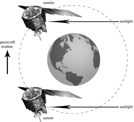
A schematic of a solar occultation measurement is shown in Fig. 1. The Sun as viewed from a satellite appears to rise and set once per orbit. Since the solar radiation is far greater than the atmospheric thermal emission, the atmospheric effect on the signal above the tropopause comes almost entirely from atmosphere absorption and scattering (extinction) of the so-lar radiation. When considering only single scattering (mul-tiple scattering, which is important in the troposphere is not considered in this study) and absorption, the atmospheric ra-diative transfer (RT) problem is greatly simplified. For this situation the broadband radiance,LS, observed by an instru-ment along the pathScan be described as:
LS=C
Z
Fig. 1. Solar occultation geometry.
whereCis a signal gain (response) constant,F is the instru-ment spectral response,J is the solar source function,τS is
the transmittance of the pathS,andν is wavenumber. For limb-paths above the atmosphere, Eq. (1) reduces toLexo:
Lexo=C Z
F (v) J (v) dv. (2)
The instrument and solar source function weighted mean transmittance along the pathScan then be defined as:
τS=LS/Lexo. (3)
Use of this ratio formulation simplifies the signal model and retrieval algorithm.
Non-local thermodynamic equilibrium (nLTE) effects are minimized by measuring spectral bands where the atmo-spheric extinction is dominated by ground state transitions. However, for some of the SOFIE channels it is necessary to account for nLTE processes in the lower thermosphere and in the vicinity of the very cold polar summer mesopause re-gion, where hot-bands contribute significantly to total band extinction (Gordley et al., 2009b). This is discussed in more detail in Sect. 6.
Retrieval of T (P ) from broadband limb-path transmit-tance measurements requires both a detailed RT model and knowledge of the atmospheric constituents that contribute to absorption and scatter of radiation along the observed path. These requirements are eliminated when using refraction measurements because retrievals based on refraction mea-surements depend only on the physics of hydrostatic balance and the relationship of refractivity to density. Limitations in using this technique with solar imaging are primarily due to errors introduced by pointing knowledge uncertainty and er-rors in upper boundary assumptions, as will be described in Sect. 6.
Retrieving temperature from broadband limb transmittance measurements requires careful attention to the physical mechanisms that produce the temperature dependence. In developing the algorithms used on HALOE and SOFIE, we investigated the major mechanisms that produce sensitiv-ity to the temperature profile. The simulations presented in this paper use the LINEPAK (Gordley et al., 1994), and BANDPAK (Marshall et al., 1994), RT models, which have been used for over 20 yr in many remote sensing missions. LINEPAK is the core RT model used in the online Spectral-Calc tool (http://www.spectralcalc.com/info/about.php). The HITRAN 2000 (Rothman et al., 2003) database is used for spectroscopic data. Note that the following simulations in-clude all isotopes contained in the HITRAN database and implicitly assume the isotopic abundances used therein. The CO2bands used in the following analyses are from SOFIE. Specifically, the 4.3 µm band is modeled using the bandpass 2259–2370 cm−1and the 2.7 µm band is modeled using the bandpass 3555–3626 cm−1(though we refer to the later band as 2.7 µm, it is centered at 2.78 µm). Also, note that HALOE has only a single CO2channel in the 2.8 µm region (3540– 3600 cm−1), similar to the SOFIE band used in the following analyses.
We begin by looking at the sensitivity of broadband ex-tinction to atmospheric temperature changes. Simulated limb extinction profiles for two CO2 bands (the SOFIE 4.3 and 2.7 µm bands) as observed through the US Standard At-mosphere are shown in Fig. 2, which also displays a typ-ical extinction profile for the 760 nm O2 A-band (12970– 13170 cm−1). Though we do not show retrieval examples for this band, we include it here to illustrate band selection considerations.
The primary physical mechanisms that cause limb-path transmittance measurements to be sensitive to atmospheric temperature are:
Fig. 2. Broadband limb-path extinction profiles for the 760 nm
O2 A-band and 2.7 and 4.3 µm CO2. Extinction is defined as
(1−τS).
2. The ideal gas law, I, stating that density is inversely proportional to temperature.
3. Atmospheric hydrostatic equilibrium, H, that couples pressure to temperature via the differential formula
dP (z)= −P (z) g(z) dz/RairT (z), (4) whereP is pressure, zis altitude, gis gravitational accel-eration, T is temperature and Rair=R∗/Mair, where R∗ is the universal gas constant andMairis the average molecular weight of the air.
Note that given a temperature profile and a defined pres-sure at one altitude, the prespres-sures at all other altitudes can be determined by integrating Eq. (4). Similarly, given a pres-sure profile and defined temperature at one altitude, the tem-perature at all other altitudes can be calculated. Maintain-ing the hydrostatic boundary condition adds complications to limb temperature retrievals, but provides an essential physi-cal constraint. A change in temperature at any altitude will change pressure at altitudes above or below depending on the direction of integration. The Earth’s atmosphere is in hydro-static equilibrium well into the lower thermosphere, butRair begins to vary at altitudes where diffusive effects become im-portant andMair changes. The work in this paper assumes thatRairis constant.
Figures 3–6 show the sensitivity results for the 4.3 and 2.7 µm CO2 bands and the 760 nm O2 A-band for a set of tangent altitudes with a vertical spacing (1z) of 2 km. A 2 km altitude spacing was found to be a good compro-mise between retrieval stability and vertical resolution. The curves labeledB,I andH show the sensitivity of limb-path extinction to a 1 K temperature change at the tangent alti-tude due only to each of the physical mechanisms discussed
Fig. 3.FLU– Sensitivity of 4.3 µm CO2limb path extinction to 1 K change at the tangent altitude, keeping layers below fixed. FLD– Sensitivity to 1 K change at the tangent point, keeping layers above fixed. F – Sensitivity to 1 K change in all layers at or above the tangent altitude, keeping layers below fixed.B– Sensitivity due to temperature used for line strength and broadening. H – Sensitiv-ity due to impact on hydrostatic pressure (hydrostatic equilibrium maintained at all altitudes).I– Sensitivity due to impact of the ideal gas law. Sensitivity is defined as the fractional change of broadband extinction through a perturbed atmosphere relative to unperturbed. In the case ofF, the perturbation is a 1 K change to all layers from the tangent point upwards. For all others, the perturbation is a 1 K change to the tangent layer alone.
above. These three curves demonstrate the competing physi-cal mechanisms that affect the measured signals. The curves labeled FLU show the total fractional change in limb-path extinction due to a 1 K perturbation at the tangent point, with pressures adjusted from the tangent point upwards to restore hydrostatic balance. This curve represents the total sensi-tivity seen by a simple reverse onion peel procedure. The reverse onion peel iterates a bottom-up retrieval until all al-titudes have converged to a stable temperature-pressure pro-file. TheFLDcurves show the sensitivity for the case where the pressures are adjusted only at the tangent level. These curves represent a traditional onion peel approach where the atmosphere is fixed above the tangent level, and thus only requires a single top-down iteration. While developing the retrieval codes used for HALOE and SOFIE, we explored a number of more complicated retrieval schemes and finally settled on the procedure depicted by the curves labeledF, which are similar toFLUexcept in this case the temperatures are perturbed for the tangent point and all points above. This procedure is similar to the bottom-up procedure described by Mill and Drayson (1978). Like the simple reverse onion peel procedure, this procedure requires iteration until all levels have converged.
Fig. 4. Same as Fig. 3 but for the 2.7 µm CO2band.
Fig. 5. Same as Fig. 3 but for O2A-band.
parts of the O2 A-band. The sensitivity curves forF are mostly positive in the stratosphere and mesosphere. Altitude regions where these curves are close to zero contain little in-formation that can be used to infer temperature. The 4.3 µm band of CO2has a broader range of usable sensitivities for
F than the 2.7 µm band. Also, as can be seen in Fig. 5, the O2A-band has little temperature sensitivity forF near 30 km and near 80 km. However, additional investigations into the temperature sensitivity of various sub-bands led to the de-termination that the long-wave side of the A-band P-branch (12985–13065 cm−1) provides very high sensitivity (Fig. 6). This is because of the much larger temperature dependence of line strength for this part of the band and exemplifies the importance of band selection.
These results demonstrate that, for all cases investigated, the scheme used by HALOE and SOFIE,F, to retrieveT (P )
from broadband transmission measurements has good sensi-tivity over a larger altitude range than the other two schemes.
Fig. 6. Same as Fig. 5 but using only the weaker part of the P-branch
of the O2A-band.
It also illustrates the relative sensitivity of each band, and demonstrates the importance of band selection. The 4.3 µm CO2band offers obvious advantages particularly in the up-per mesosphere and lower thermosphere as does the partial P-branch of the O2A-band. We are not aware of any satellite remote sensing projects that have successfully used broad-band measurements in the vicinity of the O2A-band for re-trieval of T (P ). Our investigations suggest that, if using a single broadband, the best results are obtained by using only the weak long-wave portion of the P-branch, well away from the P-branch center.
Fig. 7. Effect of lower boundary (34 km) temperature and pressure
errors on temperature retrieved from 4.3 µm CO2. Solid lines are re-trievals without boundary layer error, and dashed lines are rere-trievals with incorrect boundary layer conditions. Right-hand panel shows the errors.
The following section describes the basic numerical proce-dure used by HALOE and SOFIE for the limb-path transmit-tance measurements in the 4.3 and 2.7 µm CO2 bands and discusses the results of simulated retrievals used to investi-gate some of the major error mechanisms.
4 Basic retrieval procedure and error mechanisms
As discussed in the previous section, the algorithm used to retrieve temperature as a function of pressure, T (P ), from HALOE and SOFIE transmittance data is expected to work well from the lower stratosphere well into the mesosphere, and for the 4.3 µm band used on SOFIE, potentially into the lower thermosphere. This section takes a closer look at the numerical procedure and investigates some of the major error mechanisms.
Using an appropriate NCEP profile as an initial guess and assuming a fixed CO2concentration, the HALOE and SOFIE retrievals begin at some specified altitude,z0, typically near 30 km. Temperature, T, and pressure, P, at and below z0 remain unaltered throughout the retrieval process. Above
z0, T and P are adjusted until the modeled transmittance profile matches the measured, while maintaining hydrostatic balance. Fixing the atmospheric conditions atz0 provides a constraint to the retrieval process but also introduces an er-ror source. Here we examine the effect of this erer-ror, along with effects of measurement noise and pointing jitter. Er-rors arising from spectroscopy, instrument model, and solar source function model are not investigated in this paper, but reliable retrievals depend on careful evaluation of these ef-fects.
Fig. 8. Same as Fig. 7 but for pressure.
The analysis in the previous section suggests that the 4.3 µm CO2band provides excellent information for temper-ature retrievals from the middle stratosphere well into the lower thermosphere. While the 2.7 µm band does not per-form quite as well, it still provides significant inper-formation into the upper mesosphere. Simulated retrievals are per-formed for the CO2 bands of interest to determine the ex-pected performance. Simulated signal profiles (1z=2 km) are constructed for each band using the LINEPAK and BANDPAK radiative transfer software to solve Eqs. (1–3). Random noise is applied to the transmittance profiles prior to performing the retrieval. These transmittance signals are then used to retrieve temperature and pressure with the algo-rithm described above,F. The retrievals start with an isother-mal atmosphere (230 K for these examples) and iterate until convergence. We begin with low noise (10−7random error on the limb-path transmittances) retrieval simulations for the standard atmosphere to assess the effect of incorrect lower boundary pressure and temperature. Figures 7–10 show the results: the lines with long dashes correspond to a 2 % pres-sure error atz0 (34 km for these simulations) and the lines with short dashes show the impact of a 5 K temperature er-ror atz0. Note that though the lower boundary errors have significant impact, the retrieval returns to the correct profile within 10 to 15 km. The 4.3 µm band (Figs. 7 and 8) is much less sensitive to boundary layer errors than the 2.7 µm band (Figs. 9 and 10), and both bands exhibit higher sensitivity to pressure error than to temperature error. Note that the pres-sure errors extend belowz0for these (and subsequent) figures becauseP (z)is recalculated using Eq. (4). The very different responses of the two bands to lower boundary pressure error suggests that we may be able to use that information in a two channel retrieval to independently retrieve lower boundary pressure. We investigate this possibility in Sect. 5.
Fig. 9. Same as Fig. 7 but for the 2.7 µm CO2band.
Fig. 10. Same as Fig. 9 but for pressure.
random transmittance error of 10−5. The dashed curve in the right hand panel for each plot shows the impact of random measurement noise while the solid curve shows the mean re-trieval error. In general these simulations support the find-ings in Sect. 3. The 4.3 µm band (Figs. 11 and 12) yields more robust temperature and pressure retrieval results and is more stable at both high and low altitudes than the 2.7 µm band (Figs. 13 and 14). The pressure results for the 4.3 band (Fig. 12) are remarkable, primarily due to the strength of the 4.3 band. Comparing these results to the sensitivities shown in Figs. 3 and 4, it is apparent that the retrievals begin to fail where the sensitivity functions begin to fall off sharply above peak altitudes.
Another source of error is instrument pointing knowledge. This is modeled as a random noise on tangent point altitudes and is often referred to as jitter. The impact of pointing jit-ter on the 4.3 µm band retrieval is demonstrated in Fig. 15, where retrievals are performed on simulated measurements with 1 and 5 arc sec jitter. For this simulation a profile with
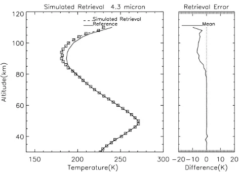
Fig. 11. Simulated temperature retrieval results for the 4.3 µm CO2 band. Right-hand panel shows the mean error and error standard deviation due to 10−5random measurement error on broadband av-eraged transmittance.
Fig. 12. Same as Fig. 11 but for pressure.
Fig. 14. Same as Fig. 13 but for pressure.
Fig. 15. Impact of random pointing error on retrieved temperature.
Right-hand panel shows the RMS difference.
significant vertical structure is used so that the impact of jitter on retrieved structure is also evaluated. These results demon-strate that pointing jitter should be less than 1 arc sec for ac-curate (<2 K error) retrievals (pointing jitter for SOFIE is less than 0.2 arc sec). Finally, the ability of the 4.3 µm re-trieval to resolve vertical profile structure is examined. Fig-ure 16 shows a simulated retrieval for an atmosphere with vertical structure on a 2 km grid. The retrieval starts with an isothermal temperature profile abovez0(30 km) and pro-ceeds with iterative application of algorithm F, the lower boundary (conditions at z0) remains fixed throughout this procedure. In this example, the initial profile is retrieved to within±2 K below 105 km, after ten retrieval iterations. For operational application, the retrieval starts from a clima-tology representative of the measurement location and fewer iterations are typically required.
As mentioned in the introduction, an assumed CO2mixing ratio is required for the 4.3 µm and 2.7 µmT (P )retrievals.
Fig. 16. The iteration sequence for a temperature profile with
sig-nificant vertical structure. Right-hand panel shows the difference from truth of retrieved profile after 10 iterations.
Fig. 17. Impact on the retrieved temperature profile of using the
CO2mixing ratio error shown in Fig. 18. Right-hand panel shows the error in retrieved temperature.
CO2 is well mixed and assumed known to within 1 % in the stratosphere and for some situations (e.g., polar sum-mer) well into the mesosphere. In the middle to upper meso-sphere, however, photo-dissociation causes variations in CO2 concentration. Thus theT (P )retrievals from HALOE and the current version (v1.03) of SOFIE, both of which assume a CO2profile, can have substantial biases in the middle to up-per mesosphere. As an example, Fig. 17 shows impact on the SOFIE 4.3 µm temperature retrieval due to an assumed error in CO2mixing ratio as shown in Fig. 18. This is not neces-sarily representative of the actual errors in SOFIE data but is meant to demonstrate the sensitivity to this type of error.
Fig. 18. CO2 mixing ratio error. Right-hand panel shows the % error.
with mostly minor impact from other constituents, but sig-nificant contributions are made by ice particles (polar meso-spheric clouds) in both bands and water in the 2.7 µm band. These are discussed briefly in Sect. 6, as are errors due to inadequate modeling of absorption line shape, nLTE effects, and instrument field-of-view (FOV).
5 Multiple channel retrieval simulations
As seen in Figs. 7–10, the 4.3 and 2.7 µm bands have very different responses to lower boundary pressure errors, which imply that this difference can be used to derive pressure in-dependent from the a-priori temperatures. Since the 2.7 µm band is more sensitive to this error, it is used in an iterative procedure to adjust the lower boundary pressure. TheF al-gorithm is used to retrieve temperature and pressure,T (P ),
from the 4.3 µm band using a simulated limb-path transmit-tance profile with 10−5transmittance error and starting from an a-priori lower boundary with 2 % pressure error and 5 K temperature error (as for Figs. 7–10). The 2.7 µm channel is then used to estimate the lower boundary pressure by simu-lating the 2.7 µm channel lower boundary measurements and iterating the pressure to achieve a match of measurement and model. These two procedures (4.3T (P ) retrieval and 2.7
Po retrieval) are iterated until the lower boundary pressure
converges. Figures 19 and 20 show the results of a simula-tion using this procedure. These results are nearly as good as the 4.3 µm retrievals with perfect lower boundary knowledge, Figs. 11 and 12.
As shown in the previous section, substantial error in re-trievedT (P )can result from inadequate knowledge of the CO2mixing ratio profile. However, with proper selection of spectral band-pass for the 2.7 and 4.3 µm channels, it is pos-sible to retrieve a CO2 mixing ratio profile simultaneously withT (P ). Simulations using the SOFIE bands show this
Fig. 19. Temperature results using a two-channel retrieval to
over-come lower boundary error of 2 % in pressure and 5 K in temper-ature. Right-hand panel shows the mean error and error standard deviation due to 10−5random measurement error on broadband av-eraged transmittance.
Fig. 20. Same as Fig. 19 but for pressure.
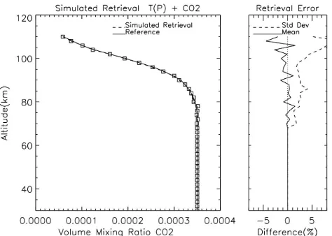
to generally be possible, however, such retrievals are more sensitive to random noise errors than theT (P )only retrieval and there are altitude regions where there is insufficient in-formation to adequately separateT (P )and CO2mixing ratio information. Figures 21–24 show retrieved profiles of tem-perature and CO2mixing ratio for a simultaneousT (P )and CO2 mixing ratio retrieval on simulated signals using the SOFIE bands. This retrieval uses theF algorithm forT (P )
Fig. 21. Temperature profile results from simultaneousT (P )and CO2mixing ratio retrieval using 2 channels in the vicinity of 4.3 and 2.7 µm with 10−5random noise. Right-hand panel shows the mean error and error standard deviation due to 10−5random measurement error on broadband averaged transmittance.
including density constraints determined from the refractive bending angle data available from SOFIE to improve these results. It is also likely that optimizing the band-pass se-lection could improve these results and that should be in-vestigated for application to future missions. Specifically, for best results, one of the bands should exhibit significantly more sensitivity to temperature than the other. Though, this is the case for the 4.3 µm band versus the 2.7 µm band used for SOFIE, there likely exists band pairs that would perform bet-ter. The results shown in Figs. 21–24 may seem inconsistent with results from Fig. 13, where the 2.7 channelT (P ) re-trieval fails above 90 km. ThisT (P )failure can be explained by instabilities near altitudes where the temperature sensitiv-ity is too small. However, in theT (P ), CO2retrieval, the 2.7 µm channel is used only for retrieving CO2 concentra-tion, and the 4.3 µm channel is used for retrieving tempera-ture. The 2.7 µm channel sensitivity to CO2is evident from
I in Fig. 4; that curve shows impact of a 1 K temperature change on density and is equivalent to the impact of less than a 1 % change in CO2concentration.
6 SOFIE approach
SOFIE is a broadband occultation sensor that employs 10 single detector channels as well as a high resolution focal plane array (FPA) that is used to track the sun. HgCdTe tectors are used to sense the 4.3 and 2.7 µm bands. The de-tector FOV for these channels at 83 km tangent point is ap-proximately 1.6 km vertical by 4.5 km horizontal with over-sampling to about 0.2 km in the vertical. More details on SOFIE, including detailed channel information, can be found at the following web-site: http://sofie.gats-inc.com/
Fig. 22. Same as Fig. 21 but retrieved CO2mixing ratio profile.
Fig. 23. Same as Fig. 21 but using 2.5×10⁻⁶random noise.
Fig. 24. Same as Fig. 23 but retrieved CO2mixing ratio profile.
The SOFIE 4.3 µm temperature retrieval algorithm uses the upward retrieval technique designated by theF curves in Fig. 3. These retrievals start at 30 km and use NCEP data to constrain the lower boundary. The retrievals operate on a 2 km vertical grid with multiple interleaves of the data com-bined to achieve the final high resolution output data. Ran-dom noise is approximately 10−5(consistent with the ran-dom error used in Figs. 11–14) providing a signal to noise ratio (SNR) of nearly 100 000 in the lower stratosphere and about 500 at 100 km.
The high resolution FPA is employed by SOFIE to pre-cisely track the Sun during an event, providing a very accu-rate measurement of the solar image as a function of altitude. Using a new technique developed for SOFIE, limb refraction profiles can be inferred to a precision of 0.02 arc sec from solar extent data determined from the measured solar image data (Gordley et al., 2009a). This precision is far better than the<0.2 arc sec jitter evident in the science channels because many pixels from the FPA are used to determine upper and lower edges of the solar image. These extremely precise re-fraction angle data are used to retrieve density profiles, which are then used to retrieveT (P )with methods similar to those described in Ward and Hermann (1998). Density is deter-mined directly from the measured refraction angle profile and
T (P )is determined from the density profile using the ideal gas law and hydrostatic integration. The details of the proce-dure used to perform these retrievals are not presented here, but we note that the primary limitations of such retrievals are pointing accuracy and upper boundary error. Pointing errors and errors in the upper boundary refraction angle lead to er-ror in the retrieved density profile, which then leads to erer-ror in retrievedT (P ). Also, retrievedT (P )is impacted by error in the upper boundary temperature.
With the precision obtained by the SOFIE refraction mea-surements, upper boundary error is the primary source of error for retrieved T (P ) in the stratosphere. The results
Fig. 25. Impact of random pointing errors and top boundary errors
on retrieved temperature, long dashed line shows impact of 5 K up-per boundary temup-perature error, short dashed lines shows impact of 5 % upper boundary error on refraction angle. Right-hand panel shows the errors, solid line in right-hand panel shows impact of ran-dom pointing error of 0.02 arc sec.
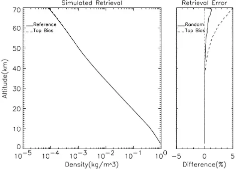
of detailed simulations are presented here to illustrate the relative importance of the various errors on retrieved den-sity and temperature. Figure 25 shows the impact of a 5 K upper boundary temperature error and a 5 % refraction an-gle error as well as uncertainty due to 0.02 arc sec random pointing error on retrieved temperature. Figure 26 shows the impact of 5 % upper boundary refraction angle error and 0.02 arc sec random pointing error on retrieved density. For SOFIE, uncertainties due to random pointing error and up-per boundary error are greatly reduced by fitting the mea-sured refraction data to reduce noise, by merging meamea-sured refraction data with refraction determined from simulation of the 4.3 µm retrievedT (P )profile using a gradual transition from about 50 km to about 70 km, and by using the 4.3 µm re-trievedT (P )to constrain the upper boundary (Gordley et al., 2009a). Starting with version 1.03 SOFIE, a refraction based retrieval is used in conjunction with the 4.3 µm retrieval to determine the final output T (P ). Version 1.03 T (P ) be-low 50 km is entirely from refraction measurements and is a combination of refraction and 4.3 µm CO2 measurements between 50 and 70 km. This approach greatly reduces up-per boundary errors for the refraction-based retrievals and also eliminates the lower boundary errors seen in Figs. 7–10. Figure 27 shows a comparison of v1.03 and v1.022 data for the period 8–14 July 2009, the mean profiles and standard deviations are determined from 83 profile pairs.
Fig. 26. Same as Fig. 25 except impact on retrieved density from
random pointing error of 0.02 arc sec and top boundary refraction angle error of 5 %.
characterization and line mixing effects in the 4.3 µm CO2 band, corrected for version 1.03. Line mixing is modeled using the AER v2.2 spectroscopic data supplied by Atmo-spheric and Environmental Research, Inc., http://rtweb.aer. com/line param frame.html. The CO2line parameters in this data are from HITRAN 2000 (Rothman et al., 2003), with the addition of line coupling parameters determined from calcu-lations using the software and database package of Niro et al. (2005).
Version 1.03 SOFIE uses CO2mixing ratio profiles from the Whole Atmosphere Community Climate Model (Garcia et al, 2007). For future SOFIE versions, we are investigat-ing use of the SOFIE 2.7 µm channel in the retrieval of CO2 mixing ratio as described in Sect. 5 with additional solution constraints provided by the refraction basedT (P )retrieval. We have not investigated use of this channel along with the 4.3 µm channel for determination of lower boundaryT (P ), also described in Sect. 5. This is primarily because of the superior information contained in the refraction data for this purpose.
The procedure used in v1.03 provides aT (P )profile with ∼2 K precision from cloud top or 5 km, whichever is higher, to 90 km. These data are currently thought to be generally accurate to within 3 K up to about 80 km, but as shown in Sect. 5, CO2 profile errors may have significant impact to as low as 60 km. And, as previously noted, ice cloud con-tamination in the polar summer mesopause region has sig-nificant contribution to total path extinction which must be addressed. SOFIE PMC measurements are used to correct for ice cloud contribution in the 4.3 µm channel. Figure 28 shows the mean impact of such correction on the tempera-ture retrieval for the 8–14 July 2009 period. The average impact is approximately 5 K at the cloud extinction peak alti-tude though thick clouds can have impact as high as 10 K. We
Fig. 27. SOFIE version 1.03 data compared to version 1.022 for
the period 8–14 July 2009. Note the difference in the 40–50 km region. Right-hand panel shows the mean difference and difference standard deviation.
currently estimate the extinction correction to be better than 20 % resulting in typically less than 2 K residual error in re-trieved temperature. Also, errors in parameters used by the CO24.3 µm nLTE model limit accuracy above 80 km. For example, error in concentration of O can have large impact above about 85 km due to its important quenching role. Like-wise, error in quenching or excitation rates can have large impact as well. Though we do not here present a detailed er-ror analysis of such effects, it should be noted that accuracy in retrievedT (P )in the lower thermosphere and in the very cold polar summer mesopause region is largely determined by accuracy of the inputs used in the nLTE model. The im-pact of such errors may approach 5 K in the polar summer mesopause region and 10 K in the lower thermosphere.
7 SOFIE results
This section discusses comparisons of version 1.03 SOFIE
Fig. 28. Impact of PMC correction, right-hand panel shows the
difference.
since observations are made year round, polar winter (PW) and equinox periods are also available for comparison. First, we choose a PS comparison period that gives numerous co-incidence profiles for all of the instruments. SABER and MLS have global coverage and typically provide excellent coincidence opportunities, but ACE is a solar occultation experiment and so provides fewer coincidence opportuni-ties. There are 3 Northern Hemisphere (NH) and 2 South-ern Hemisphere (SH) PS periods that are available for all four datasets. We have selected a period that has the most coincidences with ACE at the heart of the PS season, the week of 8–14 July 2009. We have also selected a PW period with numerous ACE coincidences, the week of 20–26 Febru-ary 2009. This period is toward the end of a dynamic period of recovery from a very intense stratospheric sudden warm-ing and the stratopause is still elevated to roughly 80 km al-titude. Figures 30 and 31 show the comparisons, the follow-ing sub-sections discuss results for each comparison dataset. These comparisons are only meant to introduce the current SOFIE results and are not meant to be a rigorous validation. A thorough validation effort is underway using more exten-sive data from new versions of the ACE (3.0) and SOFIE (1.1) data currently being processed. Also, note that a repro-cessing of the SABER data is planned for late 2011 and more extensive comparisons will be made when those data become available.
7.1 Comparisons to SABER
For this comparison we compare the most recent production version, 1.07, of the SABER data to version 1.03 SOFIE. The temperature product for this version of SABER data is dis-cussed in Remsberg et al. (2008). SABER, unlike SOFIE, is an emission experiment that uses atmospheric emission orig-inating primarily from theν2 band of CO2to deriveT (P ). These data sets therefore have independent instrument
char-Fig. 29. SOFIE tangent-point latitudes.
acteristics, rely on different measurement techniques (4.3 µm transmission vs. 15 µm emission), and use different analy-sis methods. For the comparisons shown in this and the following sections, profile pairs were selected with a max-imum latitude difference of 2◦, maximum longitude differ-ence of 20◦, and maximum time difference of 4 h. Fig-ure 30 gives comparisons of mean SOFIE temperatFig-ure mea-surements (the solid black curve in the left hand panel) to coincident profiles from SABER (red curves), for the period 8–14 July 2009. These comparisons are for 70 coincidence profiles with mean latitude difference of 0.8◦, mean longi-tude difference of 5.4◦, and mean time difference of 40 min. The SOFIE and SABER mean profiles generally agree very well (±3 K) over the range 0.1–100 mb for the high lati-tude (∼67 N) summer data shown in Fig. 30. As reported in Remsberg et al. (2008), the SABER profiles over this al-titude range have approximately 1–2 K precision but may be biased 2–3 K warm in the lower stratosphere and 1–3 K cold in the upper stratosphere to lower mesosphere (for conditions where the stratopause is in the typical 1 mb region). As stated previously, SOFIET (P )has approximately 2 K uncertainty over this altitude range so the agreement seen in Fig. 30 is within the combined uncertainties.
Fig. 30. Comparison between mean SOFIE (black), SABER (red),
ACE (green), and MLS (blue) profiles for coincident Northern Hemisphere (NH) data for the period 8–14 July 2009, left-hand panel shows the mean profiles, right-hand panel shows the mean difference and difference standard deviation profiles (SOFIE – each of the others).
at elevated altitudes until approximately mid-March. In-terestingly, SABER and SOFIE both exhibit the elevated stratopause at about 0.005 mb (MLS and ACE show it at about 0.01 mb). For both periods, the differences at pressures below 0.01 mb can be large and are likely due to among other things, CO2profile differences, accumulated pressure errors, O concentration differences (needed by the nLTE models), and different atmospheric dynamics in the coincidence pairs (a larger problem for the high latitude winter comparisons in Fig. 31). For SOFIE data with strong PMC contamination, there may also be error of 1–2 K in the 80–85 km region due to residuals in the ice cloud correction.
7.2 Comparisons to ACE
SOFIE is compared to version 2.2 of the ACE dataset. Ver-sion 3.0 is in production at this time, and a more complete comparison using this updated dataset will be carried out in the near future. The temperature product for ACE ver-sion 2.2 is discussed in Sica et al. (2008). ACE is a solar occultation sensor, but rather than the broadband measure-ments used by SOFIE, ACE derives temperature from its Fourier Transform Spectrometer (FTS) instrument that cov-ers the spectral region 750 to 4400 cm−1. The atmospheric temperature and pressure retrieval uses micro-windows that are primarily attenuated by CO2 absorption. As described in Sica et al. (2008), the ACE temperature data can exhibit large unphysical vertical oscillations in the mesosphere and to a lesser extent in the stratosphere. These oscillations ap-pear to be caused by retrieval artifacts that will be addressed
Fig. 31. Comparison between mean SOFIE (black), SABER (red),
ACE (green), and MLS (blue) profiles for coincident Northern Hemisphere (NH) data for the period 20–26 February 2009, left-hand panel shows the mean profiles, right-left-hand panel shows the mean difference and difference standard deviation profiles (SOFIE – each of the others).
uses more grid points in its analysis. MLS is a microwave instrument that uses emission from the O2 line at 118 GHz to retrieveT (P )at the altitudes compared in this paper. In general, the MLS temperatures have a precision of 1.0–2.5 K over this altitude range and systematic errors of 2–3 K with an oscillatory vertical structure. This is a known problem with instrument gain and is expected to be corrected in a fu-ture version of the AURA MLS data. The systematic errors may be worse for some situations, as exemplified in the parisons performed here. Figures 30 and 31 show the com-parisons of MLS (blue curves) to SOFIE (short-dashed black curve in the left hand panels, largely obscured by the solid curve). The comparisons in Fig. 30 are for 82 coincidence profiles with mean latitude difference of 0.3◦, mean longi-tude difference of 9.8◦, and mean time difference of 3.2 h. The comparisons in Fig. 31 are for 87 coincidence profiles with mean latitude difference of 0.4◦, mean longitude differ-ence of 7.9◦, and mean time difference of 3.3 h. Ignoring the anomalous results in the 0.5 to 2 mb region, the Febru-ary comparisons shown in Fig. 31 are very good, within 3 or 4 K up to about 0.01 mb. The MLS data shows a reformed stratopause at about 0.01 mb, similar to the 0.012 mb seen for ACE. The July comparisons shown in Fig. 30 are also gen-erally good over the same pressure range if the region from 0.2 to 3 mb is excluded. Though the data from 0.2 to 3 mb is not as obviously anomalous as that seen in the February data, it does fit the description of the biases due to the gain errors described in Schwartz et al. (2008). As for the other comparisons, differences below 0.01 mb can be large.
8 Summary
The success of the HALOE and SOFIE experiments demon-strate that broadband solar occultation measurements can be used to accurately retrieve atmosphericT (P )profiles. For this paper we presented some subtleties inherent in such re-trievals and discussed the procedures used in the HALOE and SOFIE data analyses. We also presented investigations of the impact of several major error mechanisms and demon-strated the high quality results that can be achieved using
Edited by: C. von Savigny
References
Bernath, P. F., McElroy, C. T., Abrams, M. C., Boone, C. D., But-ler, M., Camy-Peyret, C., Carleer, M., Clerbaux, C., Coheur, P. F., Colin, R., DeCola, P., DeMazi`ere, M., Drummond, J. R., Du-four, D., Evans, W. F. J., Fast, H., Fussen, D., Gilbert, K., Jen-nings, D. E., Llewellyn, E. J., Lowe, R. P., Mahieu, E., Mc-Connell, J. C., McHugh, M., McLeod, S. D., Michaud, R., Midwinter, C., Nassar, R., Nichitiu, F., Nowlan, C., Rins-land, C. P., Rochon, Y. J., Rowlands, N., Semeniuk, K., Si-mon, P., Skelton, R., Sloan, J. J., Soucy, M.-A., Strong, K., Trem-blay, P., Turnbull, D., Walker, K. A., Walkty, I., Wardle, D. A., Wehrle, V., Zander, R., and Zou, J.: Atmospheric Chemistry Experiment (ACE): mission overview, Geophys. Res. Lett., 32, L15S01, doi:10.1029/2005GL022386, 2005.
Garcia, R. R., Marsh, D. R., Kinnison, D. E., Boville, B. A., and Sassi, F.: Simulations of secular trends in the mid-dle atmosphere, 1950–2003, J. Geophys. Res., 112, D09301, doi:10.1029/2006JD007485, 2007.
Gordley, L. L., Marshall, B. T., and Chu, D. A.: LINEPAK: al-gorithms for modeling spectral transmittance and radiance, J. Quant. Spectrosc. Ra., 52(5), 563–580, 1994.
Gordley, L. L., Burton, J. C., Marshall, B. T., McHugh, M. J., Deaver, L. E., Nelsen, J., Russell III, J. M., and Bailey, S.: High precision refraction measurements by solar imaging during oc-cultation: results from SOFIE, Appl. Optics, 48(25), 4814–4825, doi:10.1364/AO.48.004814, 2009a.
Gordley, L. L., Hervig, M. E., Fish, C., Russell III, J. M., Bailey, S., Cook, J., Hansen, S., Shumway, A., Paxton, G. J., Deaver, L. E., Marshall, B. T., Burton, J. C., Magill, B., Brown, C., Thomp-son, R. E., and Kemp, J.: The solar occultation for ice experi-ment, J. Atmos. Sol.-Terr. Phy., 71(3–4), 300–315, 2009b. Hervig, M. E., Russell III, J. M., Gordley, L. L., Drayson, S. R.,
Stone, K., Thompson, R. E., Gelman, M. E., McDermid, I. S., Hauchecorne, A., Keckhut, P., McGee, T., Singh, U. N., and Gross, M. R.: Validation of temperature measurements from the halogen occultation experiment, J. Geophys. Res., 101(D6), 10277–10285, 1996.
stratospheric major warming, Geophys. Res. Lett., 36, L12815, doi:10.1029/2009GL038586, 2009.
Marshall, B. T., Gordley, L. L., and Chu, D. A.: BANDPAK: Al-gorithms for modeling broadband transmission and radiance, J. Quant. Spectrosc. Ra., 52(5), 581–599, 1994.
McCormick, M. P., Zawodny, J. M., Veiga, R. E., Larsen, J. C., and Wang, P. H.: An overview of SAGE I and II ozone measure-ments, Planet. Space Sci., 37(12), 1567–1586, 1989.
Mertens, C. J., Mlynczak, M. G., Lopez-Puertas, M., Winter-steiner, P. P., Picard, R. H., Winick, J. R., Gordley, L. L., and Russell III, J. M.: Retrieval of mesospheric and lower thermo-spheric kinetic temperature from measurements of CO215 µm Earth limb emission under non-LTE conditions, Geophys. Res. Lett., 28(7), 1391–1394, doi:10.1029/2000GL012189, 2001. Mill, J. D. and Drayson, S. R.: A nonlinear technique for inverting
limb absorption profiles, in: Remote Sensing of the Atmosphere: Inversion Methods and Applications, edited by: Fymat, A. L. and Zeuev, V. E., Elsevier, New York, 123–135, 1978.
Niro, F., Jucks, K., and Hartmann, J.-M.: Spectra calcula-tions in central and wing regions of CO2 IR bands. IV : Software and database for the computation of atmospheric spectra, J Quant Spectrosc Radiat Transfer, 95, 469–481, doi:10.1016/j.jqsrt.2004.11.011, 2005.
Remsberg, E. E., Marshall, B. T., Garcia-Comas, M., Krueger, D., Lingenfelser, G. S., Martin-Torres, J., Mlynczak, M. G., Rus-sell III, J. M., Smith, A. K., Zhao, Y., Brown, C., Gordley, L. L., Lopez-Gonzalez, M. J., Lopez-Puertas, M., She, C. Y., Tay-lor, M. J., and Thompson, R. E.: Assessment of the quality of the retrieved temperature versus pressure profiles in the mid-dle atmosphere from TIMED/SABER, J. Geophys. Res., 113, D17101, doi:10.1029/2008JD010013, 2008.
Rothman, L. S., Barbe, A., Benner, D. C., Brown, L. R., Camy-Peyret, C., Carleer, M. R., Chance, K., Clerbaux, C., Dana, V., Devi, V. M., Fayt, A., Flaud, J.-M., Gamache, R. R., Gold-man, A., Jacquemart, D., Jucks, K. W., Lafferty, W. J., Mandin, J.-Y., Massie, S. T., Nemtchinov, V., Newnham, D. A., Perrin, A., Rinsland, C. P., Schroeder, J., Smith, K. M., Smith, M. A. H., Tang, K., Toth, R. A., Vander Auw-era, J., Varanasi, P., and Yoshino, K.: The HITRAN molecu-lar spectroscopic database: edition of 2000 including updates through 2001, J. Quant. Spectrosc. Radiat. Transfer, 82, 5–44, doi:10.1016/S0022-4073(03)00146-8, 2003.
Russell III, J. M., Gordley, L. L., Park, J. H., Drayson, S. R.,
Hes-doi:10.1029/2007JD008783, 2008.
Sica, R. J., Izawa, M. R. M., Walker, K. A., Boone, C., Petelina, S. V., Argall, P. S., Bernath, P., Burns, G. B., Catoire, V., Collins, R. L., Daffer, W. H., De Clercq, C., Fan, Z. Y., Firanski, B. J., French, W. J. R., Gerard, P., Gerding, M., Granville, J., Innis, J. L., Keckhut, P., Kerzenmacher, T., Klekociuk, A. R., Kyr¨o, E., Lambert, J. C., Llewellyn, E. J., Manney, G. L., McDer-mid, I. S., Mizutani, K., Murayama, Y., Piccolo, C., Raspollini, P., Ridolfi, M., Robert, C., Steinbrecht, W., Strawbridge, K. B., Strong, K., Stbi, R., and Thurairajah, B.: Validation of the At-mospheric Chemistry Experiment (ACE) version 2.2 tempera-ture using ground-based and space-borne measurements, Atmos. Chem. Phys., 8, 35–62, doi:10.5194/acp-8-35-2008, 2008. Ward, D. M. and Herman, B. M.: Refractive sounding by use of
satellite solar occultation measurements including an assessment of its usefulness to the stratospheric aerosol and gas experiment program, Appl. Optics, 37, 8306–8317, 1998.
Waters, J. W., Read, W. G., Froidevaux, L., Jarnot, R. F., Cofield, R. E., Flower, D. A., Lau, G. K., Pickett, H. M., San-tee, M. L., Wu, D. L., Boyles, M. A., Burke, J. R., Lay, R. R., Loo, M. S., Livesey, N. J., Lungu, T. A., Manney, G. L., Nakamura, L. L., Perun, V. S., Ridenoure, B. P., Shippony, Z., Siegel, P. H., Thurstans, R. P., Harwood, R. S., and Filip-iak, M. J.: The UARS and EOS microwave limb sounder ex-periments, J. Atmos. Sci., 56, 194–218, 1999.