and Truthful Reporting of a Qualitative Sensitive Attribute
Housila P. Singh
School of Studies in Statistics
Vikram University Ujjain (M.P), India-456010 [email protected]
Tanveer Ahmad Tarray School of Studies in Statistics
Vikram University Ujjain (M.P), India-456010 [email protected]
Abstract
In this paper, a simple and obvious procedure is presented that allows to estimate the population proportion possessing sensitive attribute using simple random sampling with replacement (SRSWR). In addition to T, the probability that a respondent truthfully states that he or she bears a sensitive character when experienced in a direct response survey. An efficiency comparison is carried out to investigate in the performance of the proposed method. It is found that the proposed strategy is more efficient than Warner’s (1965) as well as Huang’s (2004) randomized response techniques under some realistic conditions. Numerical illustrations and graphical representations are also given in support of the present study.
Keywords: Randomized response technique, Direct response, Estimation of proportion, Privacy of respondents, Sensitive characteristics, Relative efficiency.
AMS Subject Classification: 62D05.
1. Introduction
A major source of bias in surveys of human populations results from the refusal of participants to cooperate and provide truthful responses, especially in cases where a question of sensitive nature is involved. To eliminate this source of bias, in estimating the proportion of a population possessing a characteristic of sensitive nature, Warner (1965)
introduced a technique termed “randomized response”. Other randomized response techniques were introduced by various other authors. These techniques either improves upon Warner’s procedure provide alternative procedures, or consider more complicated situations, for example allow unequal probabilities of selection. One can mention the work Fox and Tracy (1986), Mangat and Singh (1990), Mangat (1994), Mahmood et al. (1998), Chua and Tsui (2000), Singh et al. (2000), Chang and Huang (2001), Huang (2004), Chang et al. (2004a,2004b), Chaudhary (2011) and Singh and Tarray (2012).
2. A brief review of randomized response models
In this section we present review of the Warner’s (1965), Direct Response (DR) procedure and Huang (2004) models.
2.1 Warner’s (1965) Models
The randomized response technique is a procedure for collecting the information on sensitive characteristics without exposing the identity of the respondent. It was first introduced by Warner (1965) as an alternative survey technique for socially undesirable or incriminating behavior questions such topics as drunk driving, tax evasion, illicit drug use, induced abortion, shop lifting, child abuse, family disturbances, cheating in exams, HIV/AIDS, and sexual behavior, etc. Instead of a DR procedure, a randomization device used to gather sample information consisting of two statements: (i) ‘I am a member of group A’ and (ii) ‘I am not a member of group A’ with probabilities P and (1-P) respectively. Following this device, the respondent selects a statement unobserved by the interviewer, and then simply gives a ‘Yes’ or ‘No’ answers in a random sample of n respondents. By the method of moments, Warner obtained an unbiased estimator of the population proportion , possessing the sensitive attribute A. He considered the maximum likelihood estimator of
5 . 0 P , ) 1 P 2 (
) P 1 ( ˆ (
ˆw
where P is the proportion of the sensitive character represented in the randomized response device and ˆ m/n, the proportion of “Yes” answers obtained from the n respondents selected by simple random sampling with replacement.
The estimator is unbiased with variance
2
) 1 P 2 ( n
) P 1 ( P n
) 1 (
(2.1)
2.2 Direct Response (DR) Procedure
Social stigma and fear of reprisals often lead respondents to give biased, misleading or even erroneous responses when approached with a direct response (DR) survey method. Even for the reason of merely unwillingness to reveal secrets to strangers, many individuals attempt to avoid certain questions put to them by interviewers. Consider a dichotomous population in which every person belongs either to a sensitive group “A” or the non – sensitive complement “Ac”. The problem of interest is to estimate the population proportion of individuals who are members of “A”. Let T be the probability that the respondents belonging to “A” report the truth. The respondents belonging to the non –sensitive group “A” have no reason to tell a lie. For a DR survey of size n, the interviewee is asked if he / she are a member of “A”. then, we have a direct estimator
, n
X ˆ
n
1 i i D
with mean square error given by , ) T 1 ( n ) 1 ( ) ˆ (
MSE D D D 2 2
where Xi = 1(0) if the ith interviewee responds “Yes(N0)” and DT, see Chang and
Huang (2001).
An interesting method for the estimation of and T is given by Huang (2004), which improves on an earlier proposal by Chang and Huang (2001). In this procedure each respondent is initially required to declare if he is in group “A” or in group “Ac”. If the respondent claims to belong to group “Ac”, Warner’s (1965) procedure is carried out.
Huang’s (2004) suggestion actually consists of a two – stage method which couples the direct question procedure and Warner’s (1965) procedure. The description of Huang (2004) model is as below.
2.3 Huang (2004) Model
In his procedure, a simple random sample of size n is drawn with replacement from a finite population. The sampled observation is required to reply to a direct query whether he / she bears “A” or not. When answering “No”, the respondent is provided with a randomization device consisting of two statements (a) “I am a member of A, and (b) I am not a member of A, with probabilities P and (1-P) respectively. It is assumed that the respondents bearing to “A” give totally honest responses under the randomized response procedure, but with probability T following the usual direct response procedure.
The probability of a ‘Yes’ response in the direct response procedure is given by
, T
1
and in the randomized response procedure by
) P 1 ( T P ) 1 P 2 ( ) 1 )( P 1 ( ) T 1 ( P
2
Huang (2004) suggested the following estimators of and T respectively as
, ) P 1 ( ˆ ˆ P ˆ ) 1 P 2 ( Tˆ and ) 1 P 2 ( ) P 1 ( ˆ ˆ P ˆ 2 1 1 H 2 1 H where ˆj, the observed proportion of “Yes” answers, is the binomial random variable
with parameters n and j, j=1,2. Huang (2004) obtained the variance of ˆH as
2 H ) 1 P 2 ( n ) T 1 )( P 1 ( P n ) 1 ( ) ˆ ( V (2.2)
and the mean square error of the estimator TˆH, up to terms of order O(n1), as
. ) 1 P 2 ( n ) T 1 ( T ) P 1 ( P n ) T 1 ( T ) Tˆ (
MSE 2 2
2
H
3. The suggested Procedure
Let a simple random sample of size n is drawn with replacement from a finite population. The sampled respondent is required to reply to a direct query whether he / she bears sensitive group “A” or not. When answering “No”, the respondent is provided with a randomization device consisting of three statements:
(i) I belong to the stigmatizing group, (ii) Yes,
(iii) No
with known probabilities p, (1-P)w and (1-P) w respectively wherew[0,1], see Singh et al. (1995). Since the respondents bearing “A” have no reason to tell a lie, it may reasonably be expected that they will be completely truthful in their answers, no matter whether a direct response or a randomized response procedure is adopted. It is assumed that the respondents belonging to sensitive group “A” give completely honest responses under the randomized response procedure, but the probability T following the conventional direct response procedure.
Under the suggested procedure, the probability of “Yes” response in the direct response procedure is given by
T
1
(3.1)
and the probability of “Yes” answer using randomization device
. w ) P 1 ( ) T 1 ( P
w
(3.2)
The estimators for and T are respectively given by
, P
w ) P 1 ( ˆ ˆ P
ˆ 1 w
w
(3.3)
,w ) P 1 ( ˆ ˆ P
ˆ P Tˆ
w 1
1 w
(3.4)
where ˆ1 and ˆw, the observed proportion of “Yes” answers, are the binomial random variable with parameters
n,1
and
n,w
. The main properties of the estimator ˆw are given in the following theorem.Theorem 1. The estimator ˆw is unbiased with the variance given by
2 w
nP
] P 2 w ) P 1 ( 1 [ w ) T 1 ( P ) P 1 ( n
) 1 ( ) ˆ (
V (3.4)
Proof. The unbiasedness follows fromE(ˆw). The variance of the estimator ˆwis given by
2
w 1 w
1 2 w
P
) ˆ ˆ ( PCov 2 ) ˆ ( V ) ˆ ( V P ) ˆ (
P (1 ) (1 ) 2 2 PnP 1 w 1 w 1 w w 1 1 2
2
2 22 P P T (1 P)w P T ( P (1 P)w)
nP
1
2 nP ] P 2 w ) P 1 ( 1 [ w ) T 1 ( P ) P 1 ( n ) 1 ( (3.5)Hence the theorem.
Theorem 2. The unbiased estimator of the variance V(ˆw)is given by
2 1 2 2 w w w P ) 1 n ( ˆ ) P 1 ( P P ) 1 n ( ) P 1 }( P ] P 2 w ) P 1 ( 1 [ w { 1 n ) ˆ 1 ( ˆ ) ˆ ( Vˆ (3.6)
Proof is simple so omitted.
To derive the MSE of Tˆ we write w d1 Pˆ1 andd2
Pˆ1ˆw (1P)w
, it follows that E(d1)PTandE(d2)P. The estimator Tˆw can then be represented as2 1 w d /d
Tˆ , and we have TE(d1)/E(d2). Further, we define the following quantities: ) d ( E ) d ( E d e and ) d ( E ) d ( E d e 2 2 2 2 1 1 1 1
assuming that |e1| < 1 so that the function (1+ e2)-1 can be validly expanded as a power
series. It can be easily checked that
2 2 1 1 2 1 T n ) 1 ( ) e ( E
,
12 2 1 1 w
2 w w 2 2 nP P 2 ) 1 ( P ) 1 ( ) e ( E ,
. T nP ) 1 ( P ) e e ( E 2 w 1 1 1 2 1 The estimation error of the estimator Tˆwcan be expressed as ). n ( o ) e e ( T T
Tˆw 1 2 P 1/2 Then we state the following theorem.
Theorem 3. The mean square error of the estimatorTˆw, up to terms of ordero(n1), is given by
2 2 2 w nP ) T 1 ( P ) P 1 ( w 1 w T ) P 1 ( n ) T 1 ( T ) Tˆ ( MSE (3.8)Proof. We have
2 w w) E(Tˆ T)
Tˆ (
MSE
)] e ( E ) e e ( E 2 ) e ( E [
T2 12 1 2 22
2 w 1 1 1 2 w w s 1 1 1 2 1 1 2 2 P } P 2 ) 1 ( P ) 1 ( { PT } ) 1 ( P { 2 T ) 1 ( n T P 2 P PT 2 T ) T 1 )( 1 ( n
T 1 w
2 w 1 w 1 2 2 1 1 2 2
P T(1 T) T (1 P) w(1 (1 P)w) P (1 T) Pn
1 2 2
2
2
w1 w(1 P) P (1 T)
nP ) P 1 ( T n ) T 1 ( T 2 2 2
Thus the mean square error of the estimator Tˆw up to terms of o(n1), is given by
2 2 2 w nP ) T 1 ( P ) P 1 ( w 1 w T ) P 1 ( n ) T 1 ( T ) Tˆ ( MSE Hence the theorem.
Theorem 4. The unbiased estimator of mean square error of the direct estimatorˆD is given by
P ) 1 n ( ˆ w ) P 1 ( 2 ) ˆ ( Vˆ ) 1 n ( ) ˆ 1 ( ˆ 2 ˆ ˆ ) ˆ ( E SˆM D 1 w 2 1 w w 1
P ˆ Pˆ
Vˆ(ˆ )P ) 1 n ( ˆ 2 ˆ ˆ w 1 w 1 2 w
1
Proof is straight forward so omitted.
4. Efficiency comparison through numerical illustration
To have tangible idea about the magnitude of the relative efficiency of the suggested procedure with respect to Huang’s (2004) and direct response procedures. We have computed the percent relative efficiencies of the proposed estimators (ˆw,Tˆw) with
respect to (ˆH,TˆH) and ˆD respectively by using the following formulae:
100}] P 2 w ) P 1 ( 1 { w ) T 1 ( P )[ P 1 ( P ) 1 ( ) 1 P 2 ( P ) T 1 )( P 1 ( P ) 1 P 2 )( 1 ( ) ˆ , ˆ ( PRE 2 2 2 2 H w (4.1)
100)}] T 1 ( P ) P 1 )( w 1 ( w { T ) P 1 [( P ) T 1 ( T ) 1 P 2 ( P ) T 1 ( T ) P 1 ( P ) 1 P 2 )( T 1 ( T ) Tˆ , Tˆ (
PRE 2 2 2
2 2 2 H w (4.2)
100}] P 2 w ) P 1 ( 1 { w ) T 1 ( P )[ P 1 ( P ) 1 ( P ) T 1 ( n ) T 1 ( T ( ) ˆ , ˆ ( PRE 2 2 2 2 D
w
Using the formulae (4.1), (4.2) and (4.3) we have computed the PRE (ˆw,ˆH), PRE
) Tˆ , ˆ
(w D and PRE (Tˆw,TˆH)for the values of P= 0.6, 0.7, 0.8; T = 0.10, 0.15, 0.20, 0.25, 0.30, w = 0.10, 0.30, 0.50, 0.70, 0.90, and = 0.1 (0.1) 0.5 and findings are displayed in Tables 1,2 and 3.
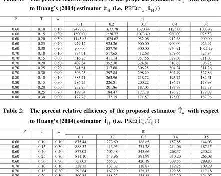
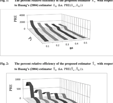
Tables 1 and 2 show that the values of RE(ˆw,ˆH) and RE(Tˆw,TˆH) are larger than 100, showing that ˆwand Tˆw are more efficient than ˆHand TˆH respectively. This fact can also be observed from Figures 1 and 2.
Tables 1 and 2 exhibit that
for fixed values of (P,T,w) the PRE (ˆw,ˆH) and PRE(Tˆw,TˆH)decrease as increases,
for fixed values of (P,w,) the PRE (ˆw,ˆH)
PRE(Tˆw,TˆH)
decreases (increases) slowly (rapidly) as T increases.Large gain in efficiency by using ˆw (Tˆw) over ˆH (TˆH) is observed when (P,w,) are closer to 0.1.
It is observed from Table 3 that:
for fixed (P,T,w) the PRE (ˆw,ˆD) increases as increases,
for fixed (P,,w), the PRE (ˆw,ˆD) decreases as T increases,
for fixed (T,w,), the PRE (ˆw,ˆD) increases as P increases.
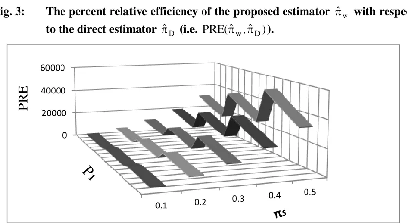
There is substantial gain in efficiency by using the proposed estimator ˆw over direct estimator ˆD for all values of (P,,T,w)considered here, See Figure 3.
Finally we conclude that the proposed procedures are superior to Huang’s (2004) procedure and hence the Chang and Huang’s (2001) procedure and the usual direct procedure.
5. Conclusion
suggested by Huang’s (2004) and the direct response procedure. We have also provided the unbiased estimator of the mean square error of the direct estimator with the help of the proposed randomized response procedure. Thus the proposed randomized response procedure is therefore recommended for use in survey sampling practice.
Acknowledgements
The authors are thankful to the Editor – in- Chief, and to the anonymous learned referee for his valuable suggestions regarding improvement of the paper.
References
1. Chang HJ and Huang KC (2001). Estimation of proportion and sensitivity of a qualitative character. Metrika, 53, 269-280.
2. Chang HJ, Wang CL and Huang KC (2004 a). On estimating the proportion of a qualitative sensitive character using randomized response sampling. Qual. Qant., 38, 675-680.
3. Chang HJ, Wang CL and Huang KC (2004 b). Using randomized response to estimate the proportion and truthful reporting probability in a dichotomous finite population. Jour. Appl. Statist., 31, 565-573.
4. Chaudhuri A (2011). Randomized response and indirect questioning techniques in surveys. CRC Press, London.
5. Chaudhuri A and Mukerjee R (1988). Randomized Response: Theory and Techniques. Marcel-Dekker, New York, USA.
6. Chua TC and Tsui AK (2000). Procuring honest responses indirectly. Jour. Statist. Plan. Inf., 90, 107-116.
7. Cochran WG (1977). Sampling Technique. 3rd Edition. New York: John Wiley and Sons, USA.
8. Fox JA and Tracy PE (1986). Randomized Response: A method of sensitive surveys. Newbury Park, CA: SEGE Publications.
9. Huang KC (2004). Survey technique for estimating the proportion and sensitivity in a dichotomous finite population. Statistica Neerlandica, 58, 75-82.
10. Mahmood M, Singh S and Horn S (1998). On the confidentiality guaranteed under randomized response sampling: a comparison with several new techniques.
Biom. Jour., 40, 237-242.
11. Mangat NS (1994). An improved randomized response strategy. Jour. Roy. Statist. Soc., B, 56 (1), 93-95.
12. Mangat NS and Singh R (1990). An alternative randomized procedure.
Biometrika, 77, 439-442.
14. Singh S and Singh R, Mangat NS and Tracy DS (1995). An improved two–stage randomized response strategy. Statistical Papers, 36, 265-271.
15. Singh S (2003). Advanced sampling theory with applications. Kluwer Academic Publishers, Dordrecht.
16. Sing S, Singh R and Mangat NS (2000). Some alternative strategies to Moor’s model in randomized response model. Jour. Statist. Plan. Inf., 83, 243-255.
17. Singh HP and Tarray TA (2012). A Stratified Unknown repeated trials in randomized response sampling. Comm. Kor. Statist. Soc., 19, (6), 751-759.
18. Singh R and Mangat NS (1996). Elements of Survey Sampling, Kluwer Academic Publishers, Dordrecht, The Netherlands.
Table 1: The percent relative efficiency of the proposed estimator ˆw with respect to Huang’s (2004) estimator ˆH (i.e. PRE(ˆw,ˆH))
P T w
0.1 0.2 0.3 0.4 0.5
0.60 0.10 0.10 2478.08 1677.78 1320.44 1125.00 1008.47 0.60 0.15 0.30 1500.00 1228.77 1073.49 980.00 925.53 0.60 0.20 0.50 1145.63 1024.62 952.08 912.68 900.00 0.60 0.25 0.70 979.12 925.26 900.00 900.00 926.97 0.60 0.30 0.90 900.00 887.76 900.00 940.91 1022.29 0.70 0.10 0.10 774.51 517.65 412.68 357.66 325.84 0.70 0.15 0.30 516.25 411.14 357.56 327.50 311.03 0.70 0.20 0.50 402.84 352.30 324.81 310.68 306.25 0.70 0.25 0.70 341.81 317.68 306.25 304.24 311.26 0.70 0.30 0.90 306.25 297.84 298.29 307.49 327.86 0.80 0.10 0.10 383.71 263.96 218.72 195.72 182.61 0.80 0.15 0.30 286.25 226.81 200.22 186.27 178.98 0.80 0.20 0.50 232.93 201.86 187.05 179.93 177.78 0.80 0.25 0.70 199.84 184.47 177.78 176.25 179.02 0.80 0.30 0.90 177.78 172.15 171.57 175.00 182.96
Table 2: The percent relative efficiency of the proposed estimator Tˆw with respect
to Huang’s (2004) estimator TˆH (i.e. PRE(Tˆw,TˆH))
P T w
0.1 0.2 0.3 0.4 0.5
0.60 0.10 0.10 675.44 273.60 188.65 157.85 144.03 0.60 0.15 0.30 888.32 413.95 271.28 214.06 187.15 0.60 0.20 0.50 877.02 505.48 343.66 268.37 230.23 0.60 0.25 0.70 811.10 543.96 391.99 310.20 265.08 0.60 0.30 0.90 757.03 555.37 420.19 338.55 289.83 0.70 0.10 0.10 228.33 137.32 118.87 112.25 109.29 0.70 0.15 0.30 292.84 167.29 135.12 122.85 117.18 0.70 0.20 0.50 300.84 188.22 148.88 132.20 124.07 0.70 0.25 0.70 281.88 196.40 157.14 138.31 128.45 0.70 0.30 0.90 259.45 195.78 160.10 140.89 130.03 0.80 0.10 0.10 143.64 112.38 106.21 104.02 103.03 0.80 0.15 0.30 169.42 121.68 110.91 106.94 105.13 0.80 0.20 0.50 175.86 127.69 114.16 108.85 106.31 0.80 0.25 0.70 167.22 128.61 114.86 108.97 106.00 0.80 0.30 0.90 153.33 125.20 112.94 107.17 104.03
Table 3: The percent relative efficiency of the proposed estimator ˆw with respect to the direct estimator ˆD (i.e. PRE(ˆw,ˆD))
P T w
0.1 0.2 0.3 0.4 0.5
Fig. 1: The percent relative efficiency of the proposed estimator ˆw with respect to Huang’s (2004) estimator ˆH (i.e. PRE(ˆw,ˆH))
Fig. 2: The percent relative efficiency of the proposed estimator Tˆw with respect
to Huang’s (2004) estimator TˆH (i.e. PRE(Tˆw,TˆH)).
0.1 0.2 0.3 0.4
0.5 0
2000 4000
PRE
0.1 0.2 0.3 0.4
0.5 0
500 1000
Fig. 3: The percent relative efficiency of the proposed estimator ˆw with respect to the direct estimator ˆD (i.e. PRE(ˆw,ˆD)).
0.1 0.2 0.3
0.4 0.5 0
20000 40000 60000