The Cryosphere, 7, 779–795, 2013 www.the-cryosphere.net/7/779/2013/ doi:10.5194/tc-7-779-2013
© Author(s) 2013. CC Attribution 3.0 License.
EGU Journal Logos (RGB)
Advances in
Geosciences
Open Access
Natural Hazards
and Earth System
Sciences
Open AccessAnnales
Geophysicae
Open AccessNonlinear Processes
in Geophysics
Open AccessAtmospheric
Chemistry
and Physics
Open AccessAtmospheric
Chemistry
and Physics
Open Access DiscussionsAtmospheric
Measurement
Techniques
Open AccessAtmospheric
Measurement
Techniques
Open Access DiscussionsBiogeosciences
Open Access Open Access
Biogeosciences
Discussions
Climate
of the Past
Open Access Open Access
Climate
of the Past
Discussions
Earth System
Dynamics
Open Access Open Access
Earth System
Dynamics
DiscussionsGeoscientific
Instrumentation
Methods and
Data Systems
Open Access
Geoscientific
Instrumentation
Methods and
Data Systems
Open Access DiscussionsGeoscientific
Model Development
Open Access Open Access
Geoscientific
Model Development
DiscussionsHydrology and
Earth System
Sciences
Open AccessHydrology and
Earth System
Sciences
Open Access DiscussionsOcean Science
Open Access Open Access
Ocean Science
Discussions
Solid Earth
Open Access Open Access
Solid Earth
DiscussionsThe Cryosphere
Open Access Open Access
The Cryosphere
Discussions
Natural Hazards
and Earth System
Sciences
Open Access
Discussions
High-resolution interactive modelling of the mountain
glacier–atmosphere interface: an application over the Karakoram
E. Collier1,2, T. M¨olg2, F. Maussion2, D. Scherer2, C. Mayer3, and A. B. G. Bush1 1Department of Earth & Atmospheric Sciences, University of Alberta, Edmonton, Canada 2Chair of Climatology, Technische Universit¨at Berlin, Berlin, Germany
3Commission for Geodesy and Glaciology, Bavarian Academy of Sciences and Humanities, Munich, Germany
Correspondence to: E. Collier ([email protected])
Received: 12 November 2012 – Published in The Cryosphere Discuss.: 4 January 2013 Revised: 9 April 2013 – Accepted: 13 April 2013 – Published: 6 May 2013
Abstract. The traditional approach to simulations of alpine glacier mass balance (MB) has been one-way, or offline, thus precluding feedbacks from changing glacier surface conditions on the atmospheric forcing. In addition, alpine glaciers have been only simply, if at all, represented in atmo-spheric models to date. Here, we extend a recently presented, novel technique for simulating glacier–atmosphere interac-tions without the need for statistical downscaling, through the use of a coupled high-resolution mesoscale atmospheric and physically-based climatic mass balance (CMB) mod-elling system that includes glacier CMB feedbacks to the atmosphere. We compare the model results over the Karako-ram region of the northwestern Himalaya with remote sens-ing data for the ablation season of 2004 as well as with in situ glaciological and meteorological measurements from the Baltoro glacier. We find that interactive coupling has a lo-calized but appreciable impact on the near-surface meteo-rological forcing data and that incorporation of CMB pro-cesses improves the simulation of variables such as land sur-face temperature and snow albedo. Furthermore, including feedbacks from the glacier model has a non-negligible effect on simulated CMB, reducing modelled ablation, on average, by 0.1 m w.e. (−6.0 %) to a total of −1.5 m w.e. between 25 June–31 August 2004. The interactively coupled model shows promise as a new, multi-scale tool for explicitly re-solving atmospheric-CMB processes of mountain glaciers at the basin scale.
1 Introduction
Spatially-distributed simulations of glacier surface and cli-matic mass balance (where the latter term denotes surface plus near-subsurface mass balance following; Cogley et al., 2011) require distributed meteorological forcing; however, obtaining these data is complicated both by the spatial and temporal scarcity of in situ observations and by the “scale mismatch” between the spatial scales represented in atmo-spheric models and those relevant for surface and climatic MB calculations (e.g. Machguth et al., 2009; M¨olg and Kaser, 2011). To overcome these issues, forcing data can be obtained by extrapolation from point measurements by au-tomated weather stations, where available, or interpolation from climate reanalyses and atmospheric model output, us-ing surface- and free-air lapse rates. Surface lapse rates ex-hibit significant spatial and temporal variability, however, leading to uncertainty in temperature downscaling from alti-tude changes (Marshall et al., 2007; Gardner et al., 2009; Pe-tersen and Pellicciotti, 2011). In addition, the assumption of linear lapse rates over glacier surfaces may be inappropriate (Petersen and Pellicciotti, 2011) and may under-predict near-surface temperature over debris-covered regions (Reid et al., 2012). Finally, additional corrections are often required for the poor representation of the strength and spatial variabil-ity of processes relevant to mass balance, such as orographic precipitation, in coarse spatial-resolution atmospheric mod-els (e.g. Paul and Kotlarski, 2010; Radi´c and Hock, 2011).
(Machguth et al., 2009; Kotlarski et al., 2010a,b; Paul and Kotlarski, 2010),∼11 km (Van Pelt et al., 2012) and∼1– 3 km grid spacings (M¨olg and Kaser, 2011; M¨olg et al., 2012a,b) as forcing for distributed alpine glacier surface- and climatic-mass-balance calculations. This approach provides high spatial- and high temporal-resolution atmospheric fields obtained from a physical model, and the increased resolution allows for improved representation of features such as com-plex topography and orographic precipitation (e.g. Maussion et al., 2011). However, most of these studies required statisti-cal corrections to link mesosstatisti-cale circulation patterns and me-teorological fields simulated by regional atmospheric models to local conditions on the glacier surface. M¨olg and Kaser (2011) first showed that, at sufficiently high spatial resolu-tion (∼1 km), a regional atmospheric model could be used to force explicit distributed simulations of glacier CMB with-out statistical corrections at the glacier–atmosphere interface. This approach has since been applied successfully in multi-ple locations for small glaciers (M¨olg and Kaser, 2011; M¨olg et al., 2012a,b).
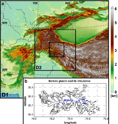
Traditional approaches to simulations of surface and cli-matic mass balance, including those discussed above, have been one-way, or offline, in which meteorological fields are passed to the CMB model but changing surface boundary conditions due to CMB processes are not fed back into the atmospheric model. Interactively or two-way coupled atmo-spheric and ice-sheet simulations with simple treatments of ablation have been performed to estimate the paleoclimate and future climate behaviours of the Laurentide and Green-land ice sheets, respectively, with significant alterations to at-mospheric circulation, temperature and precipitation result-ing from ice sheet evolution (Ridley et al., 2005; Pritchard et al., 2008). Although an initial effort has been made to in-clude “interactive” alpine glaciers in a regional atmospheric model with the subgrid-scale parameterization of Kotlarski et al. (2010b), the influence of two-way coupling on the at-mospheric forcing and explicitly simulated surface and cli-matic mass balance has yet to be assessed for alpine glaciers. Here, we build on a new, unified and explicit approach to resolving the glacier–atmosphere interface without statistical downscaling (M¨olg and Kaser, 2011), through the use of an interactively coupled high-resolution mesoscale atmospheric and physically based CMB modelling system. By allowing changes in glacier surface conditions to feed back on the at-mospheric drivers, the model provides a consistent calcula-tion of surface energy and mass fluxes. For the initial applica-tion of the coupled model, we simulate the Karakoram region of the northwestern Himalaya (Fig. 1), which is estimated to contain anywhere from∼1250–4000 km3of ice, covering an area of∼18 000 km2(Bolch et al., 2012). Due to its exten-sive glaciation, this region presents a high potential influence on atmospheric simulations resulting from the inclusion of feedbacks from alpine glaciers. In addition, Yao (2007) esti-mates that more than half of the glaciated area is contained in the 15 largest glaciers, thus optimizing the Karakoram
Fig. 1. (a) WRF atmospheric model domains, configured with
hor-izontal spatial resolutions of 33, 11, and 2.2 km. Terrain elevation from the GTOPO30 dataset is shaded in units of meters. (b) Outline of Baltoro glacier and its tributaries, which are included in WRF D3, with the mean stake locations labeled and denoted by stars.
for representation in a high-resolution atmospheric model, where the smallest practical grid spacing is on the order of a few kilometers.
The Karakoram is also of interest due to recent evidence of stable or positive mass balances (e.g. Hewitt, 2005; Scherler et al., 2011; Gardelle et al., 2012; K¨a¨ab et al., 2012), which contrasts with the general trend of mass loss exhibited by glaciers elsewhere in the Himalaya (Cogley, 2011). However, definitive statements about the mass balance of Karakoram glaciers have been hampered by a dearth of both in situ mea-surements and information on ice thickness changes. The lat-ter limitation has been partially addressed by recent geodetic studies (Gardelle et al., 2012; K¨a¨ab et al., 2012) that support reduced mass loss or even a positive mass balance anomaly in the early 21st century but emphasize the spatial and tempo-ral heterogeneity of recent glacier behaviour. In addition, ex-plicit, physically based, spatially distributed numerical mod-elling has the potential to clarify the dynamics occurring in this region.
boundary layer on the atmospheric forcing, and (2) assess the ultimate influence of interactive coupling on simulations of glacier mass balance. A final goal of this work is to im-prove the representation of alpine glaciers in mesoscale at-mospheric models by introducing additional, relevant physi-cal processes.
2 Methodology
The coupled modelling system (hereafter “WRF-CMB”) consists of two components: the advanced research version of the nonhydrostatic and fully compressible Weather Re-search and Forecasting (WRF) mesoscale atmospheric model version 3.4 (Skamarock and Klemp, 2008, Sect. 2.1) and the process-based surface-energy and CMB model of M¨olg et al. (2008, 2009, 2012a, Sect. 2.2). The CMB model has been incorporated into the WRF source code as an additional physics option, and, thus, the user may select via runtime (“namelist”) options whether the CMB simulation is offline (conventional one-way forcing, with feedbacks only from WRF’s land surface model) or interactive (feedback from CMB model to WRF over glaciated grid cells; Sect. 2.3). We performed two simulations, one interactive (INT) and one offline (OFF), for the months of June–August 2004, to coincide with a limited number of glaciological and mete-orological measurements from the Baltoro glacier available for evaluation (Sect. 2.4), with the period of 1–25 June dis-carded as model spin-up time. Here we use the term interac-tive to denote surface–atmosphere exchanges through heat, moisture and momentum fluxes only and not through topo-graphic feedbacks, as glacier geometry is held constant over our brief simulation. As a first approximation, we focused on the meteorologically driven fluctuations of mass balance and neglected the influence of debris cover.
2.1 Mesoscale atmospheric model
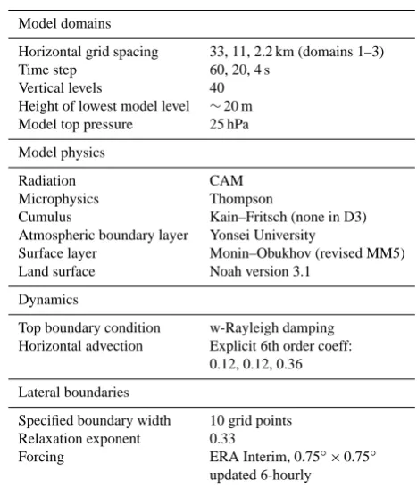
For these simulations, WRF was configured with three nested domains of 33, 11 and 2.2 km spatial resolution, centered over the northwestern Himalaya (D1–3; Fig. 1). By increas-ing the spatial resolution over the region of interest, the use of multiple grid nesting improves the representation of com-plex terrain and associated processes such as orographic pre-cipitation, and has been found to increase the simulation skill of WRF for mountain summit conditions (M¨olg and Kaser, 2011). Model physics and other settings were selected fol-lowing the recommendations of the National Center for At-mospheric Research (NCAR) for regional climate simula-tions with WRF (Table 1; outlined in WRF ARW user’s guide). Note that no cumulus parameterization was employed in the highest-resolution, convection-permitting model do-main, WRF D3 (e.g. Molinari and Dudek, 1992; Weisman et al., 1997). The range of terrain elevation represented in this domain at 2.2 km resolution is 916 to 7442 m a.s.l.,
Table 1. WRF configuration.
Model domains
Horizontal grid spacing 33, 11, 2.2 km (domains 1–3) Time step 60, 20, 4 s
Vertical levels 40 Height of lowest model level ∼20 m Model top pressure 25 hPa
Model physics
Radiation CAM Microphysics Thompson
Cumulus Kain–Fritsch (none in D3) Atmospheric boundary layer Yonsei University
Surface layer Monin–Obukhov (revised MM5) Land surface Noah version 3.1
Dynamics
Top boundary condition w-Rayleigh damping Horizontal advection Explicit 6th order coeff:
0.12, 0.12, 0.36
Lateral boundaries
Specified boundary width 10 grid points Relaxation exponent 0.33
Forcing ERA Interim, 0.75◦×0.75◦ updated 6-hourly
which encompasses the most heavily glaciated altitudes in the Karakoram (∼2700–7200 m, as shown in Fig. S2 of Bolch et al. (2012), with the mean basin-wide glacier ele-vation located at 5326 m).
In this study, WRF was coupled with the Noah land surface model (LSM; Chen and Dudhia, 2001). The land-ice mask was updated using glacier outlines for the Karakoram region based on the glacier inventory of China (Shi et al., 2009) as well as inventories generated by ICIMOD (2007) and GlobGlacier (Frey et al., 2012). Other modifications made to glaciated grid cells included assigning (1) zero vegetation cover, (2) maximum and minimum albedo values consistent with the parameterization in the CMB model (Sect. 2.2), and (3) a soil moisture availability of 1.0 (from an original value of 0.95). The conventional bulk computation of the latent heat flux in the WRF surface module is multiplied by the last parameter; therefore, this change was made for consistency with the CMB model.
The atmospheric model was forced with ERA-Interim data at 0.75◦×0.75◦ spatial-resolution and 6-hourly
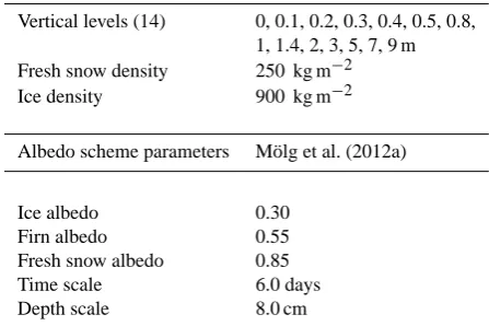
Table 2. MB model configuration.
Vertical levels (14) 0, 0.1, 0.2, 0.3, 0.4, 0.5, 0.8, 1, 1.4, 2, 3, 5, 7, 9 m Fresh snow density 250 kg m−2 Ice density 900 kg m−2
Albedo scheme parameters M¨olg et al. (2012a)
Ice albedo 0.30 Firn albedo 0.55 Fresh snow albedo 0.85 Time scale 6.0 days Depth scale 8.0 cm
SSM/I and MODIS Snow Cover SWE data (Brodzik et al., 2007), assuming a snow density of 300 kg m−2and assign-ing an initial depth of 2 m over large glaciers where these data are missing (less than 0.1 % (8 in total) of data points in the region spanned by WRF D1).
WRF employs a terrain-following hydrostatic-pressure co-ordinate in the vertical, defined as eta (η) levels (Skamarock and Klemp, 2008). For these simulations, the lowest atmo-spheric model level was specified atη=0.997585 (∼20 m) to maintain the validity of the constant-flux assumption in the bulk computation of the turbulent heat fluxes, as the sur-face mid-layer height (less than 10 m) is used in the calcula-tion following the approach of the Noah LSM. We selected the recently revised Monin–Obukhov surface layer (Jim´enez et al., 2012), which was found to improve the simulation of the diurnal amplitudes of near-surface meteorological fields over complex terrain with a horizontal spatial resolution of 2 km. We also used positive-definite explicit 6th order dif-fusion (Knievel et al., 2007), in order to dampen grid-scale noise in the atmospheric fields and because M¨olg and Kaser (2011) found this option improved the simulated magnitude of precipitation at high elevations on Kilimanjaro. For the simulations presented here, we selected the default value of the diffusion coefficient (0.12) for all model domains except D3, for which we used a value of 0.36. The choice of the dif-fusion parameter value is uncertain; sensitivity runs revealed that increasing the strength increased simulated precipitation at high elevations, which may be attributable to increased dif-fusive transport, with the best agreement with the Urdukas AWS data found for the selected value.
2.2 Surface energy and mass balance model
The CMB model is described fully by M¨olg et al. (2008, 2009) with the most recent updates in M¨olg et al. (2012a), but we will review some important features here. The model computes the column specific mass balance from solid pre-cipitation, surface deposition and sublimation, surface and subsurface melt, and refreeze of both meltwater and liquid
precipitation. To determine the mass fluxes, the model first solves the surface energy balance equation:
S↓·(1−α)+L↓+L↑+QS+QL+QG+QPRC=FNET (1) in which the terms correspond to, from left to right: incoming short-wave radiation, broadband albedo, incoming and out-going long-wave radiation, turbulent fluxes of sensible and latent heat, ground heat flux and heat flux from precipitation. The ground heat flux, QG, consists of a conductive compo-nent (QC) as well as a compocompo-nent due to subsurface pene-tration of short-wave radiation (QPS). The net flux,FNET, represents the energy available for melt, QM, provided the surface temperature is at the melting point,TM=273.15 K.
The model treats both surface and subsurface processes, including surface albedo and roughness evolution based on snow depth and age; snowpack compaction and densification by refreeze; and the influence of penetrating solar radiation, refreeze and conduction on the englacial temperature distri-bution. The CMB model is forced by air temperature, hu-midity, wind speed, and air pressure, all of which were taken from the lowest model level (z=20 m). Note that the diag-nostically updated 2 and 10 m meteorological fields were not used as forcing so as to (1) be consistent with the approach of the Noah LSM (Chen and Dudhia, 2001), and (2) prevent decoupling of the atmosphere and land surface, wherein the lower atmosphere is no longer influenced by surface condi-tions. The CMB model also takes as input: total precipitation and its frozen fraction; incoming short- and long-wave ra-diation; and time between snowfall events. Some model pa-rameter values are provided in Table 2. The initial subsurface temperature was specified through linear interpolation of the input data to the Noah LSM, available at 0.1, 0.4, 1.0, and 2.0 m depths, and assigning a constant value of 268.6 K be-low this level. The be-lower boundary is specified at 268.6 K during the simulation, based on measurements taken from a Tibetan glacier (M¨olg et al., 2012a). We address uncertain-ties in the subsurface temperature initialization by including a long (25 day) model spin-up period.
2.3 Coupling architecture
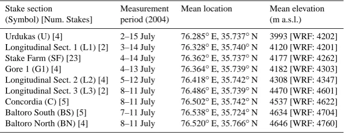
Table 3. Summary of available ablation stake measurements from the Baltoro glacier.
Stake section Measurement Mean location Mean elevation (Symbol) [Num. Stakes] period (2004) (m a.s.l.)
Urdukas (U) [4] 2–15 July 76.285◦E, 35.737◦N 3993 [WRF: 4202] Longitudinal Sect. 1 (L1) [2] 3–14 July 76.328◦E, 35.740◦N 4120 [WRF: 4201] Stake Farm (SF) [23] 4–14 July 76.362◦E, 35.737◦N 4177 [WRF: 4262] Gore 1 (G1) [4] 4–13 July 76.364◦E, 35.739◦N 4182 [WRF: 4303] Longitudinal Sect. 2 (L2) [4] 5–12 July 76.418◦E, 35.742◦N 4308 [WRF: 4347] Longitudinal Sect. 3 (L3) [2] 8–11 July 76.486◦E, 35.739◦N 4470 [WRF: 4601] Concordia (C) [5] 8–11 July 76.502◦E, 35.742◦N 4537 [WRF: 4622] Baltoro South (BS) [5] 7–11 July 76.538◦E, 35.724◦N 4634 [WRF: 4704] Baltoro North (BN) [4] 8–11 July 76.520◦E, 35.766◦N 4646 [WRF: 4760]
Sect. 1. The incorporation of the CMB model for all glacier grid points in the coupled model adds negligible computa-tional expense to WRF simulations.
For interactive simulations, the CMB model updates over glaciated areas in WRF, at every time step: (1) surface heat and moisture fluxes, (2) surface and subsurface (including deep soil) temperature, (3) snow depth, water equivalent and fractional cover, (4) surface albedo and roughness, and (5) surface specific humidity. The inclusion of feedbacks rep-resents a more consistent approach, as it permits the near-surface forcing variables to be modified by exchanges of mass, momentum and moisture between the glacier and the atmospheric surface layer. In this study, the CMB model out-put accumulated energy and mass fluxes every hour that were then converted into hourly averages for analysis; these data will be referred to as “hourly”.
As indicated at the beginning of Sect. 2, it is not abso-lutely correct to label the two forcing approaches as “offline” and “interactive” because the atmospheric model currently receives surface feedbacks through the Noah LSM. There have been recent efforts to improve the simulation of snow processes in WRF, such as with the introduction of the Noah-MP land surface parameterization (Niu et al., 2011), which, for example, introduces separate vegetation canopy and sur-face layers and the possibility of multiple vertical layers in the snowpack. However, the simplified treatment of glacier grid cells in the Noah LSM is retained. Thus, by incorporat-ing the CMB model, we are able to simulate more physical processes relevant for glaciers, such as refreezing of meltwa-ter in the snowpack, englacial melt, and formation of super-imposed ice. Other improvements to the treatment of snow and ice physics, compared with the Noah LSM, include intro-ducing multiple layers in the snowpack, increasing the col-umn depth from 2 to 9 m, consideration of snow porosity, and allowing for full snowpack ablation to expose bare ice. The latter point is especially critical, as the Noah LSM im-poses minimum snow depth and water equivalent values over land-ice grid cells.
2.4 Measurements for model evaluation
In Sect. 3.2, we compare the coupled model results with a limited number of available ablation stake measurements as well as automated weather station (AWS) data that were acquired in summer 2004 on the Baltoro glacier (35◦350– 35◦560N, 76◦040–76◦460E; Mihalcea et al., 2006). The glacier is approximately 62 km long, with an average (maxi-mum) width of 2.1 (3.1) km (Mayer et al., 2006). Therefore, in WRF-CMB the Baltoro glacier is represented by at least one grid point in the along-glacier direction and we resolve longitudinal rather than transverse gradients in surface con-ditions. We use data from 6 sections (SF, U, G1, C, BN, and BS) as well as from longitudinal transects along the glacier (L1, L2 and L3), comprising 53 stakes in total that provide sufficient spatial coverage (cf. Figs. 1b or 4b) to evaluate both the spatial pattern and the magnitude of ablation in the coupled model applied to the Baltoro glacier. The ablation measurements were taken at different intervals between 1– 15 July 2004; a brief summary of the location and other de-tails of the stake measurements are given in Table 3 (a more detailed description of the data can be found in Mihalcea et al., 2006). While the data represent a brief period, they provide the only available direct ablation measurements in the Karakoram. For the comparison, total simulated surface lowering was interpolated to the mean location of the stake section or transect using inverse distance weighting.
The AWS was situated adjacent to the glacier on a moraine ridge at an elevation of 4022 m (35◦43.6840N, 76◦17.1640E) and provided hourly mean data after 18 June 2004 (Mihalcea et al., 2006). We compared these data with WRF data from the nearest model grid point (located at an elevation of 4322 m), which was also non-glaciated and therefore was more consistent in the land sur-face type. However, the data therefore do not include direct feedbacks from the CMB model. Note that the assumptions discussed in Sect. 2.1 for snow initialization were not applied over the stake sites on the main glacier area (cf. Fig. 1b).
using MODIS/Aqua (1) MYD10A1 daily snow albedo avail-able at 500 m resolution, and (2) MYD11A2 eight-day land surface temperature available at 1 km resolution, with daily data obtained by averaging day- and night-time temperatures where both fields were available and were assigned the high-est quality assurance flag for MODIS products. Due to the prevalence of missing data in the snow albedo dataset, we considered only the grid cells with at least 25 % valid obser-vations during the 67 day period for comparison with WRF. Both MODIS datasets were re-projected to the WRF D3 grid before completing the analysis.
3 Results and discussion
We first compare our simulated results with remote sensing data (Sect. 3.1) and with meteorological and glaciological measurements from the Baltoro glacier (Sect. 3.2). The role of interactive coupling on the atmospheric forcing data and on simulations of CMB will then be discussed. Results are presented from the finest-resolution atmospheric model do-main only, since it provides the most realistic terrain repre-sentation.
3.1 Remote sensing data
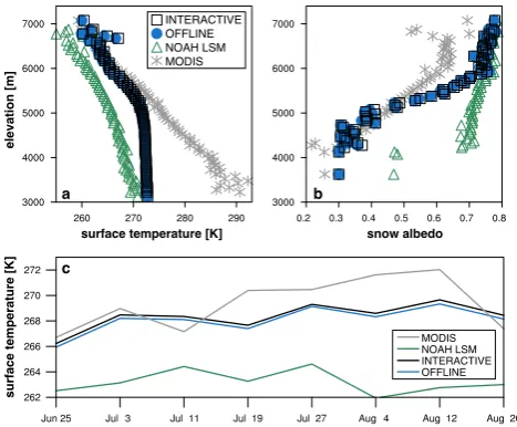
Figure 2 presents a comparison between WRF-CMB and the MODIS/Aqua datasets discussed in Sect. 2.4. The ele-vational profile of land surface temperature (LST) averaged over the simulation period produced by the CMB model is in good agreement with the MODIS data above∼5200 m and is an improvement on the Noah LSM values at all re-solved elevations (Fig. 2a). The strong divergence of mod-elled and observed LST below 5200 m likely results from neglecting debris cover, since its presence allows the glacier surface to be warmed by solar radiation above the melt-ing point. Supraglacial debris extent has also been found to increase with distance down glacier in remote-sensing case studies of the central Karakoram (e.g. Scherler et al., 2011). Specific to the Baltoro glacier and its tributaries, Mayer et al. (2006) found that debris coverage increased to 70–90 % of the glacier area below 5000 m, with 100 % coverage found below the U site (Fig. 1b). A time-series analysis of LST, averaged only over elevations greater than 5200 m is presented in Fig. 2c. The CMB model gives an im-proved performance over the LSM alone, although LST is generally under-predicted, with mean biases of−1.0,−1.3, and−6.1 K in the INT, OFF, and Noah LSM simulations, respectively. Conversely, snow albedo in WRF-CMB is in good agreement with MODIS below∼5200 m (Fig. 2b), al-though simulated values are constrained by the lower bound ofαice=0.3 as snow depth goes to zero and, thus, slightly overestimate the observational values at the lowest eleva-tions. Above 5200 m, WRF-CMB over-predicts snow albedo compared with MODIS. However, it produces values and an
surface temperature [K]
surface temperatur
e [K]
snow albedo
elevation [m]
b a
c
INTERACTIVE OFFLINE NOAH LSM MODIS
MODIS NOAH LSM INTERACTIVE OFFLINE
Fig. 2. Comparison between WRF-CMB D3, Noah LSM, and
MODIS for land surface temperature, (a) averaged from 25 June– 28 August 2004, and in 50 m elevation bins; (c) the mean time series above 5200 m elevation; and for (b) snow albedo, averaged between 25 June–31 August 2004, over glacier grid cells where at least 25 % of the daily times are available.
altitudinal gradient that are in much better agreement with observations than the Noah LSM.
The strong discrepancy between Noah LSM and MODIS data is in part related to the treatment of grid cells defined as glacial ice: the LSM in WRF v3.4 imposes minimum val-ues of snow depth and water equivalent of 0.5 and 0.1 m, respectively, thus preventing the exposure of bare ice or de-bris and the associated lowering of surface albedo. In addi-tion, the Noah LSM employs a time-decaying snow albedo formulation (based on the scheme of Livneh et al., 2009) and determines surface albedo using fractional snow cover to cor-rect a background snow-free albedo. Although snow albedo is likewise an exponential function of age in the CMB model (following Oerlemans and Knap, 1998), the actual surface albedo also depends on snow depth to account for surface darkening when the snowpack is thin. It is clear from Fig. 2 that this formulation, in combination with permitting snow-free conditions, gives more realistic values.
a
b
c
d
e
Jun 25 Jul 2 Jul 9 Jul 16 Jul 23 Jul 30 Aug 6 Aug 13 Aug 20 Aug 27 Jun 25 Jul 2 Jul 9 Jul 16 Jul 23 Jul 30 Aug 6 Aug 13 Aug 20 Aug 27 Jun 25 Jul 2 Jul 9 Jul 16 Jul 23 Jul 30 Aug 6 Aug 13 Aug 20 Aug 27
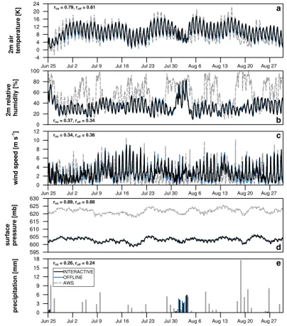
Fig. 3. Hourly (a) air temperature at 2 m, (b) relative humidity at 2 m, (c) wind speed at 10 m, and (d) surface air pressure, as well as (e)
daily total precipitation. Solid black (blue) curves display data from the interactive (offline) simulations while the dashed grey curve is the Urdukas AWS station data. Note the difference in elevation of the AWS (4022 m a.s.l.) and the terrain height in the closest WRF grid cell (4322 m).
3.2 Baltoro glacier
Figure 3 presents a time series of modelled and observed near-surface meteorological data from the Urdukas AWS that is situated adjacent to the Baltoro glacier. WRF-CMB is skill-ful in simulating air temperature at 2 m, and its evolution over the study period, including capturing periods of reduced di-urnal variability at the beginning and between 30 July and 6 August. However, the good agreement in near-surface tem-perature despite a difference in real and modelled elevation of
Table 4. Ablation rates (cm day−1) and debris thickness on the Bal-toro glacier.
Average Mean debris Site INT OFF measured (ice) thickness (cm) U −5.6 −5.5 −3.9 8.6 L1 −5.4 −5.3 −3.5 7.0 SF −5.2 −5.1 −4.3 3.8 G1 −5.2 −5.1 −2.9 18.0 L2 −5.1 −5.1 −4.8 2.5 L3 −5.0 −4.9 −4.3 2.0 C −4.9 −4.9 −2.9 6.0 BS −6.4 −5.6 −1.8 6.8 BN −7.4 −7.7 −1.8 7.8
cycle is smaller in WRF-CMB, which may be attributable to differing thermal properties of the real and modelled land surface or to the fact that the AWS sensor was not aspirated. The magnitude of the near-surface wind speed is also in agreement with the AWS data (Fig. 3c). However, an im-portant discrepancy is the underestimation of precipitation at this particular grid cell in both INT and OFF simulations: the AWS records a total of 122.8 mm of precipitation be-tween 25 June and 31 August, while INT and OFF simulate 46.9 and 48.4 mm, respectively (Fig. 3e). Missing precipi-tation events are also reflected as discrepancies in the time series of relative humidity (cf. Fig. 3b, e) and are consistent with an overestimation of incoming short-wave radiation as a result of too little cloud cover. The disagreement in mea-sured and simulated humidity and precipitation may reflect several sources of error, such as in the forcing data at the lat-eral boundaries. In addition, the spatial resolution of WRF D3 may be insufficiently fine to fully resolve orographic up-lift or microscale complex flow features that affect precip-itation at the AWS. Furthermore, we do not use a cumulus parameterization in the finest model domain and therefore as-sume that convection is explicitly resolved. However, previ-ous studies indicate that a grid spacing on the order of 100 m (Bryan et al., 2003; Petch, 2006) or even 10 m (Craig and D¨ornback, 2008) is needed to capture the dominant length scales of moist cumulus convection. A final potential error source is the difference in the land surface type adjacent to the AWS and model grid cell: the Baltoro glacier is debris-covered at the Urdukas site, while WRF-CMB has a clean snow/ice surface. The differing thermal properties of the ad-jacent surface area, specifically the limiting of temperature at the melting point in WRF-CMB, may also contribute to differences in localized convection.
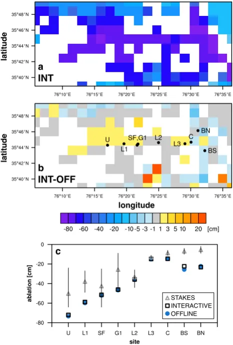
WRF-CMB produces 40 to 80 cm of ablation along the main body of the Baltoro glacier between 1–15 July 2004 (Fig. 4a). Spatial comparison of the two simulations re-veals only small differences, generally on the order of a few centimetres, consistent with the short nature of the study period (Fig. 4b). There are slightly positive anomalies at
[cm] a
INT
b INT-OFF
c
STAKES INTERACTIVE OFFLINE
latitude
longitude
latitude
Fig. 4. (a) Total and (b) INT-OFF surface height change between
1–15 July 2004, in the vicinity of the main tongue of the Baltoro glacier. Stake site and transect locations shown in (b), with ad-ditional information provided in Table 3. White grid cells corre-spond to non-glaciated area. (c) Measured mean ablation (triangles) at stake locations, with range of observed values denoted by bars. Simulated INT (OFF) ablation shown by black squares (blue cir-cles).
a
b
c
d
e
f
g
h
air temperature [°C]
relative humidity [%]
winds [m s
-1]
precipitation [mm]
incoming shortwave [Wm
-2
]
incoming long wave [Wm
-2
]
pressure [hPa]
frozen fraction
of precipitation
for all plots INTERACTIVE OFFLINE 4
3 2 1 0 -1
mean diurnal cycle
hour [°C]
Jun 25 Jul 9 Jul 23 Aug 6 Aug 20
Jun 25 Jul 9 Jul 23 Aug 6 Aug 20
Jun 25 Jul 9 Jul 23 Aug 6 Aug 20
Jun 25 Jul 9 Jul 23 Aug 6 Aug 20
Jun 25 Jul 9 Jul 23 Aug 6 Aug 20 Jun 25 Jul 9 Jul 23 Aug 6 Aug 20
Jun 25 Jul 9 Jul 23 Aug 6 Aug 20
date [mon dd] date [mon dd]
Fig. 5. Daily mean (a) air temperature, (b) relative humidity, (c) wind speed, (d) total precipitation, incoming (e) normal short-wave and (f)
downward long-wave radiation at ground surface, (g) air pressure, and (h) frozen fraction of precipitation, area-averaged over all glaciated grid cells. Data for (a–c), and (g) are taken from the lowest model level (z=20 m). The subpanel in (a) presents the average diurnal temperature cycle over the simulation period. Black (blue) curves display data from the interactive (offline) simulation.
refreeze than in OFF), with the strongest improvement at BS. The improvement at this site stems from faster com-plete snow cover removal (∼1 day earlier in INT), which reduces subsurface penetration of short-wave radiation and, thus, subsurface melt production. Finally, the overestimation of ablation by WRF-CMB tends to diminish as the observa-tion period increases (Fig. 4d), which then suggests that the coupled model as configured in this study may be best suited for “climatological” simulations of glacier mass balance due to its sensitivity to the timing of precipitation.
Mihalcea et al. (2008) performed distributed surface-energy sub-debris melt modelling, using the Urdukas AWS
model also includes additional processes, such as snowpack ablation and surface vapour fluxes, that bring the total sim-ulated mass loss to 0.078 km3 w.e. between 1–15 July. We employ the same glacier outline, that of Mayer et al. (2006); however, discrepancies in our estimates may arise from its projection to the WRF D3 grid, differences in removal of tributary glaciers, and the coarser representation of the Bal-toro glacier at 2.2 km spatial resolution (vs. 90 m in Mihalcea et al., 2008). Despite these and other sources of disagree-ment, comparing the two estimates gives an approximate measure of the effect of neglecting debris, which is thought to cover 38 % of the Baltoro glacier (Mayer et al., 2006) and 73 % of the altitude range of the main glacier tongue consid-ered in Mihalcea et al. (2008), in our simulations.
3.3 Influence of interactive coupling
Figure 5 presents a time series of daily means of the near-surface WRF meteorological data used as forcing for the CMB model and provides the context for the fluctuations of surface energy and mass fluxes discussed in this section. Near-surface air temperatures in INT are higher by 0.3◦C on average than in OFF (Fig. 5a). The difference arises pri-marily from a reduced amplitude of the diurnal cycle, with higher nocturnal temperatures (Fig. 5a subpanel). INT sim-ulates higher surface temperatures (Tsfc), as well as higher subsurface temperatures in the top 0.5–1 m (peak differences are∼0.7◦C, not shown), as a result of stronger downward long-wave radiative forcing (see Fig. 5f for daily average curves). The increase in L↓ is expressed between evening and early morning and is a direct result of higher mixing ratios at 2 m in INT (not shown). The change in radiative forcing in INT translates into less heat extraction from the surface layer, through a reduced nocturnal QS, and, in turn, into the near-surface temperature difference. Note that the near-surface air temperature evolution simulated in INT may represent an improvement, as M¨olg et al. (2012b) found that WRF+Noah LSM can produce an excessively large diurnal cycle as a result of a nighttime cold bias at 2 m compared with AWS measurements on Kilimanjaro. Inter-active coupling also results in a reduction of mean incom-ing short-wave radiation (−9.0 W m−2) and, as previously mentioned, a mean increase in incoming long-wave radia-tion (2.4), changes that arise from alteraradia-tions to atmospheric clouds and moisture (see Fig. 6). Basin-scale daily-mean dif-ferences in the other forcing variables for the CMB model are negligible.
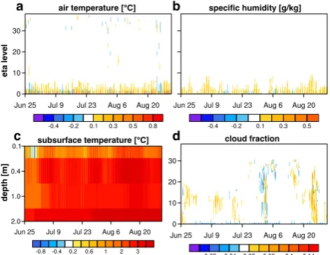
The atmospheric changes induced by including feedbacks from the CMB model are generally small in magnitude and limited in vertical extent, but still appreciable. Air tempera-ture and mixing ratio anomalies are generally confined to the lowest 10 model levels, which correspond to the layer be-tween a mean surface pressure of 543 hPa and the level of 450 hPa (Fig. 6a). Vertical changes in the mean cloud cover fraction are variable, with the greatest differences present
air temperature [°C] specific humidity [g/kg]
subsurface temperature [°C] cloud fraction
eta level
depth [m]
a b
c d
Fig. 6. Vertical and subsurface distribution of the influence of
inter-active coupling over glaciated areas illustrated by hourly time series of the change (INT-OFF) in area-averaged (a) air temperature,(b) specific humidity, (c) subsurface temperature, and (d) cloud frac-tion.
near the levels of 375 (η=12–14) and 125 hPa (η=26–29; Fig. 6d). However, interactive coupling has a strong warm-ing influence on the subsurface temperature distribution (on average,+2.6 K; Fig. 6c), as a result of (1) the inclusion of the energy flux from penetrating solar radiation, and (2) the method for updating deep soil temperature (Tds), which is de-fined at a depth of 3 m. With regard to the latter point,Tdsin INT is taken from the CMB model subsurface scheme, which resolves the column to a depth of 9 m but is constrained by a lower boundary temperature of 268.6 K in this study. In contrast, the Noah LSM updatesTds using a weighted com-bination of the annual meanTsfcof the previous year and of the last 150 days as the data become available, with no lower threshold imposed. The resulting minimum values forTsfcin the CMB model and Noah LSM are∼245 and 224 K, re-spectively.
The non-negligible influence of interactive coupling on the near-surface meteorological forcing data translates primarily into reduced ablation of snow and ice in INT (Fig. 7a and b). Area-averaged modelled surface height lowering is smaller and total mass balance is less negative in INT, with a mean reduction in ablation over the Karakoram basin of 0.1 m w.e. (−6.0 %), to a cumulative value of−1.5 m w.e. by 31 Au-gust. The difference in the total mass balance arises despite higherTsfcin INT (Fig. 7c). The inclusion of additional pro-cesses, such as the refreezing of meltwater, and the differ-ent method of subsurface temperature calculation both con-tribute to higherTsfcin both INT and OFF compared with the Noah LSM.
a
b
surface height change [cm]
mass balance [kg m
-2]
surface temperature [K]
c
NOAH INTERACTIVE OFFLINE
Fig. 7. Daily basin-scale averages of (a) accumulated surface height
change, (b) accumulated total mass balance, and (c) surface tem-perature. Black (blue) curves display data from the interactive (of-fline) simulation. For reference, surface temperature simulated by the Noah LSM is the dashed grey curve in (c).
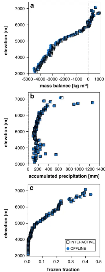
distribution is characterized by a shallowing of the VBP above∼5000 m, associated with (1) an increase in the pos-itive vertical gradient of the fraction of solid precipitation that contributes positively to CMB (Fig. 8c), and (2) cooling of mean surface temperature with height to below the melt-ing point (cf. Fig. 2a). Above 5875 m, the VBP profile again steepens as a result of large increases in accumulated, solid precipitation. Below 5875 m, INT produces less ablation (on average, 117.7 mm w.e.), while above this level it simulates a mean increase in accumulation (13.4) in part due to small in-creases in both accumulated precipitation and its frozen frac-tion (cf. Fig. 8b and c). Averaged over the whole period, the equilibrium line altitudes are 5469 and 5536 m in INT and OFF, respectively, which exceed the annual and generalized estimate of 4500 m by Hewitt (2005) and of 4200–4800 m by Young and Hewitt (1993), because we only simulate the ablation season.
Figure 9 presents the surface fluxes of energy and mass from the interactive simulation. On average, the main en-ergy sources are incoming radiation,S↓(374.3 W m−2) and
L↓ (220.4), with smaller contributions from QS (9.5) and QC (8.1; Fig. 9a). The main energy sinks are outgoing
mass balance [kg m-2]
a
frozen fraction
c
INTERACTIVE OFFLINE accumulated precipitation [mm]
b
70006000
5000
4000
3000
7000
6000
5000
4000
3000 7000
6000
5000
4000
3000
elevation [m]
elevation [m]
elevation [m]
0.0 0.1 0.2 0.3 0.4 0.5 0 200 400 600 800 1000 1200 1400 -5000 -4000 -3000 -2000 -1000 0 1000
Fig. 8. (a) The vertical mass balance profile of the Karakoram basin
at the end of the simulation. The altitudinal dependence of (b) total accumulated precipitation, and (c) mean frozen fraction, averaged over the simulation. Data are area-averaged in 50 m elevation bins.
0.64 0.56 0.46 0.40
daily mean energy fluxes [W m
-2]
daily total mass fluxes [kg m
-2]
Jun 25 Jul 2 Jul 9 Jul 16 Jul 23 Jul 30 Aug 6 Aug 13 Aug 20 Aug 27
Jun 25 Jul 2 Jul 9 Jul 16 Jul 23 Jul 30 Aug 6 Aug 13 Aug 20 Aug 27
a
b
albedo
L
S
L S
Fig. 9. From the interactive WRF-CMB simulation: daily (a) mean surface energy balance components (left y-axis; see Eq. 1 for explanation
of symbols) and albedo values (grey right y-axis), and (b) sums of mass fluxes. The radiation variables are shown in (a) as solid (directed downward) and dashed (upward) lines, albedo as grey dots, and the other surface energy fluxes as bars. The heat flux from precipitation (QPRC) is negligible and not shown. Values are averaged over glaciated grid cells only.
the snowfall event that occurs at the beginning of August (cf. solid precipitation bars in Fig. 9b) is clearly associated with (1) a reduction inS↓and an increase inL↓, (2) a spike in both surface albedo and thusS↑, and (3) a reduction in ab-sorbed short-wave radiation that translates into reduced en-ergy for surface and subsurface melt. Furthermore, changes in glacier surface conditions have a noticeable feedback on the atmosphere during and after the snowfall event (cf. e.g.
S↓in Fig. 5e or cloud fraction changes in Fig. 6d).
Interactive coupling has the strongest influence on the net short-wave and ground heat fluxes in the atmospheric model (Fig. 10a). The average QG in INT (−23.7 W m−2) greatly exceeds that simulated by the Noah LSM alone (−0.5), due to (1) the inclusion of penetrating short-wave radiation, which always represents an energy sink at the surface, and (2) higher surface temperatures, which result in a stronger (more negative) flux downward to the subsurface. Mean ab-sorbed short-wave radiation is also much larger in INT (184.8
vs. 107.9), as a result of lower average surface albedo (0.49 vs. 0.71; see Fig. 2c) over the simulation period. Smaller changes in the turbulent heat fluxes reflect in part different treatments of surface roughness, which is a spatially and tem-porally varying parameter in WRF-CMB that ranges between 0.8 and 2.6 mm as a function of snow age and generally ex-ceeds the constant value of 1 mm specified by the Noah LSM for snow/ice surfaces.
In the CMB model, interactive coupling induces the largest magnitude change in the net short-wave (−3.3 %,) and long-wave (+1.8 %,) radiative fluxes, as a result of the changes to
∆INT-OFF mass fluxes [kg m-2]
WRF
a
CMB
b
c
CMB
∆INT-OFF surface energy fluxes [W m-2] ∆INT-OFF surface energy fluxes [W m-2]
Fig. 10. Area-averaged mean difference (INT−OFF) over the sim-ulation period and over glaciated grid cells of (a) the main compo-nents of the WRF surface energy budget, (b) the MB model energy fluxes, and (c) the MB model mass fluxes. Symbols in (a) repre-sent, from left to right, net short- and long-wave radiation, ground heat flux, and turbulent fluxes of sensible and latent heat. Note that the sign convention for the turbulent fluxes in (a) is opposite to (b). Symbols in (b) are discussed in Sect. 2.2
(M¨olg et al., 2008). The reduction in the turbulent heat fluxes appears to stem from reduced 10 m wind speeds (−0.2 to 4.3 m s−1), due to the surface roughness changes discussed above. The changes also occur despite (1) a weaker cor-rection for atmospheric stability on average, according to a modified version of the Monin–Obukhov stability function (Eq. 12 in Braithwaite, 1995); and (2) stronger mean gradi-ents in vapor pressure (1VP; −1.2 in INT vs.−0.7 hPa in OFF) and temperature (1T; 1.8 vs. 1.2 K) between the near-surface and lower boundary.
The net result is a decrease of 4.8 % in the average energy available for surface melt, QM, and less negative mass bal-ance over the INT simulation (cf. Fig. 7b). The difference is primarily reflected in a reduction in surface melt (−5.8 %; Fig. 10c), and is compounded by increases in both refreez-ing in the snowpack and the formation of superimposed ice (8.5 % combined) as well as by greater solid precipitation (4.0 %). In general, mass exchanges between the glacier sur-face and the overlying boundary layer are smaller in INT, with the weakening in QL resulting in less sublimation (par-ticularly at night) and deposition (at all times).
3.4 Remarks and perspectives for future research
The explicit approach to modelling alpine glacier climatic mass balance using WRF first demonstrated by M¨olg and Kaser (2011) has been applied in offline mode for simula-tions of small glaciers (M¨olg and Kaser, 2011; M¨olg et al., 2012a,b) and has yielded important insights into the physi-cal processes and the atmospheric forcing underlying mass fluctuations. However, here we demonstrate that feedbacks due to CMB processes are evident for the heavily-glaciated Karakoram region. The basin-scale influence of interactive coupling on the atmospheric forcing data, while moderate, acts to reduce the energy available for surface melt and, in concert with both reduced mass exchanges between the sur-face and boundary layer and increased refreezing, reduces modelled ablation during the summer of 2004. Furthermore, we demonstrate that the inclusion of additional real processes such as CMB feedbacks renders WRF-CMB capable of sim-ulating observed magnitudes of CMB.
To the best of our knowledge, only one previous study, that of Kotlarski et al. (2010b), has performed interactive and dis-tributed simulations of alpine glacier mass balance, achieved by introducing a subgrid-scale parameterization for glaciers and their areal changes into a regional climate model config-ured with a relatively coarse spatial resolution of∼18 km. However, their implicit treatment “pools” the glaciers located in a grid cell into one ice mass at a fixed altitude and with a uniform snow depth. Furthermore, they quantify the effect of two-way coupling by comparing their interactive simula-tion with a control run that contains no glaciers (i.e. snow and ice surfaces are compared with bare soil or vegetation-covered surfaces), thus obscuring the exact role of feedbacks. Therefore, this paper presents the first assessment of the im-portance and strength of interactions between alpine glaciers and the atmosphere on explicit simulations of CMB.
the greatest test for some of the simplifying assumptions em-ployed, such as zero debris cover. However, a longer ap-plication is needed to assess the year-long and inter-annual influence of interactive coupling, as well as the long-term performance of the atmospheric model under the climate-simulation forcing strategy we employ (i.e. with no nudging or model re-initialization; e.g. Maussion et al., 2011). Simu-lations of glacier mass balance are also inherently sensitive to the modeled solid precipitation (M¨olg and Kaser, 2011), which is influenced in our study by the choice of micro-physics scheme. Furthermore, the optimal choice of diffu-sion scheme, its strength, and its influence on simulated pre-cipitation and therefore glacier CMB are beyond the scope of this paper and have not been investigated fully for our area of interest and model configuration. The simulation of near-surface meteorological fields by WRF over glacier sur-faces has been found to be relatively insensitive to the choice of physical parameterizations (Claremar et al., 2012); how-ever, the extent to which modelled CMB is dependent on the model physics, the choice of numerics, and the spatial resolu-tion of the finest domain represents an important uncertainty that will be explored in a future study.
The mean proportion of debris covered-area on Karakoram glaciers is estimated to be 18–22 % (Scherler et al., 2011; Hewitt, 2011), which is higher than the pan-Himalayan av-erage of∼10 % (Bolch et al., 2012). Specific to the Bal-toro glacier, Mayer et al. (2006) estimate that∼38 % of the total glacier area is debris covered. The presence of debris above a threshold, or “critical thickness”, of∼2 cm has been shown, empirically and through surface energy balance mod-elling, to reduce glacier ablation as a result of its insulating effect (e.g. Østrem, 1959; Kayastha et al., 2000; Nicholson and Benn, 2006; Reid et al., 2012). The range of mean de-bris thicknesses at the stake sites is 2.0–18.0 cm (Table 4), suggesting that on the whole insulation effects should dom-inate over the lowering of surface albedo except at the sites L2 and L3 where debris thickness is approximately equal to the critical value. Indeed modelled ablation closely matches the measured rate at these two sites and elsewhere is overes-timated by WRF-CMB (Fig. 4c), physically consistent with the exclusion of debris in this study. This interpretation is supported by the first distributed ablation modelling study for debris-covered ice, that of Reid et al. (2012), which found re-duced sub-debris ablation when depth exceeded 2 cm. How-ever, it is noteworthy that geodetic estimates of early 21st century elevation changes in the Karakoram (Gardelle et al., 2012; K¨a¨ab et al., 2012) do not show a difference between clean and debris-covered ice.
Given the similarity of the underlying surface types in INT (snow/ice) and OFF (snow) influencing the atmospheric forcing data, the difference in simulated CMB for the clean glacier simulations is relatively small. From the results pre-sented here, it could be expected that the inclusion of feed-backs is not essential for small glaciers or less glaciated basins. However, we would expect the interactive inclusion
of the CMB model to have a larger influence for glaciers with significant debris cover, as its presence alters surface temperature and moisture properties and thus turbulent ex-changes with the surface boundary layer (e.g. Takeuchi et al., 2000). To assess the role of feedbacks for debris-covered glaciers and to allow the WRF-CMB modelling system to provide long-term, accurate simulations in the Karakoram, including the effects of debris cover on surface conditions and glacier ablation represents important future work. Treat-ing debris cover in distributed mass balance modellTreat-ing is also becoming more important in light of observations of increas-ing debris-covered area in many regions (e.g. Stokes et al., 2007; Bhambri et al., 2011). Another process that is thought to be important for Karakoram glaciers is accumulation via snow and ice avalanching (e.g. Hewitt, 2011), which may be useful to parameterize. Finally, dynamical ice flow changes have been shown to be important when quantifying the re-sponse of Himalayan glaciers to climate fluctuations on mul-tiannual timescales (e.g. Scherler et al., 2011; Gardelle et al., 2012; K¨a¨ab et al., 2012; Azam et al., 2012).
4 Conclusion
CMB feedbacks have been introduced into a new, multi-scale modelling approach for explicitly resolving the surface and climatic mass balance processes of alpine glaciers, and this technique has been extended to the regional scale. Although validation data is sparse, the model captures the magnitude of available in situ measurements, with improvements aris-ing from includaris-ing feedbacks from the CMB model to WRF. Furthermore, discrepancies between observed and simulated ablation can be attributed to physical processes neglected as simplifying assumptions, particularly debris cover effects.
Both components of WRF-CMB are based on physical principles, with no statistical downscaling at their interface. The direct linkage increases the applicability of this approach for the simulation of the past- and future-climate response of glaciers, since the modelling system produces a physically-consistent response to changes in external forcing. Incorpo-ration of the CMB model also increases the number of phys-ical processes important for glaciers represented in the at-mospheric model, and provides a consistent calculation of surface energy and mass fluxes, since changes in glacier sur-face conditions are permitted to influence the atmospheric drivers. Perhaps the most important advantage, however, is that WRF-CMB permits direct causal attribution of glacier mass changes to both physical processes and the main at-mospheric drivers. With further development, the model has the potential to bridge the data gap in the Karakoram and shed light on the role of climate forcing in the anomalous behaviour of glaciers in this region.
alpine glaciers simply as a boundary condition. We suggest that this unified, explicit approach should be increasingly adopted in future studies, particularly for heavily glaciated regions.
Acknowledgements. E. Collier was supported by a Natural Sci-ences and Engineering Research Council of Canada (NSERC) CGS-D award, a NSERC Michael Smith Foreign Study Schol-arship, and an Alberta Ingenuity Graduate Student Scholarship. T. M¨olg was supported by the Alexander von Humboldt Founda-tion. F. Maussion and D. Scherer acknowledge support from the German Research Foundation (DFG) Priority Programme 1372 under the code SCHE 750/4-3, and the German Federal Ministry of Education and Research (BMBF) Programme CAME under the code 03G0804A. A.B.G. Bush acknowledges support from NSERC and from the Canadian Institute for Advanced Research. The supercomputing resources for this study were provided by Compute/Calcul Canada. The authors thank Ev-K2-CNR for providing the meteorological data from the Baltoro glacier, together with the University of Milan for supporting the field work. They would also like to thank V. Radic and two anonymous reviewers for their constructive comments.
Edited by: V. Radic
References
Azam, M. F., Wagnon, P., Ramanathan, A., Vincent, C., Sharma, P., Arnaud, Y., Linda, A., Pottakkal, J. G., Chevallier, P., Singh, V. B., and Berthier, E.: From balance to imbalance: a shift in the dynamic behaviour of Chhota Shigri glacier, western Hi-malaya, India, J. Glaciol., 58, 315–324, 2012.
Bhambri, R., Bolch, T., Chaujar, R. K., and Kulshreshtha, S. C.: Glacier changes in the Garhwal Himalaya, India, from 1968 to 2006 based on remote sensing, J. Glaciol., 57, 543–556, 2011. Bolch, T., Kulkarni, A., K¨a¨ab, A., Huggel, C., Paul, F., Cogley, J. G.,
Frey, H., Kargel, J. S., Fujita, K., Scheel, M., Bajracharya, S., and Stoffel, M.: The state and fate of Himalayan glaciers, Science, 336, 310–314, 2012.
Braithwaite, R. J.: Aerodynamic stability and turbulent sensible-heat flux over a melting ice surface, the Greenland ice sheet, J. Glaciol., 41, 562–571, 1995.
Brodzik, M. J., Armstrong, R., and Savoie, M.: Global EASE-Grid 8-day Blended SSM/I and MODIS Snow Cover, National Snow and Ice Data Center, Boulder, Colorado, USA, Digital media, 2007.
Bryan, G. H., Wyngaard, J. C., and Fritsch, J.: Resolution require-ments for simulations of deep moist convection, Mon. Weather Rev., 131, 2394–2416, 2003.
Chen, F. and Dudhia, J.: Coupling an advanced land surface-hydrology model with the Penn State – NCAR MM5 modelling system. Part I: Model implementation and sensitivity, Mon. Weather Rev., 129, 569–585, 2001.
Claremar, B., Obleitner, F., Reijmer, C., Pohjola, V., Waxeg˚ard, A., Karner, F., and Rutgersson, A.: Applying a mesoscale at-mospheric model to Svalbard glaciers, Adv. Meteorol., 2012, 321649, doi:10.1155/2012/321649, 2012.
Cogley, J. G.: Present and future states of Himalaya and Karakoram glaciers, Ann. Glaciol., 52, 69–73, 2011.
Cogley, J. G., Hock, R., Rasmussen, L. A., Arendt, A. A., Bauder, A., Braithwaite, R. J., Jansson, P., Kaser, G., M¨uller, M., Nicholson, L., and Zemp, M.: Glossary of Glacier Mass Balance and Related Terms, IHP-VII Technical Documents in Hydrology No. 86, IACS Contribution No. 2, UNESCO-IHP, Paris, 2011. Craig, G. C. and D¨ornback, A.: Entrainment in cumulus clouds:
What resolution is cloud-resolving?, J. Atmos. Sci., 65, 3978– 3988, 2008.
Dee, D. P., Uppala, S. M., Simmons, A. J., Berrisford, P., Poli, P., Kobayashi, S., Andrae, U., Balmaseda, M. A., Balsamo, G., Bauer, P., Bechtold, P., Beljaars, A. C. M., van de Berg, L., Bidlot, J., Bormann, N., Delsol, C., Dragani, R., Fuentes, M., Geer, A. J., Haimberger, L., Healy, S. B., Hersbach, H., Hlm, E. V., Isaksen, L., K˚allberg, P., K¨ohler, M., Matricardi, M., McNally, A. P., Monge-Sanz, B. M., Morcrette, J.-J., Park, B.-K., Peubey, C., de Rosnay, P., Tavolato, C., Thpaut, J.-N., and Vitart, F.: The ERA-Interim reanalysis: configuration and perfor-mance of the data assimilation system, Q. J. Roy. Meteorol. Soc., 137, 553–597, 2011.
Frey, H., Paul, F., and Strozzi, T.: Compilation of a glacier inven-tory for the western Himalayas from satellite data: methods, chal-lenges, and results, Remote Sens. Environ., 124, 832–843, 2012. Gardelle, J., Berthier, E., and Arnaud, Y.: Slight mass gain of Karakoram glaciers in the early twenty-first century, Nat. Geosci., 5, 322–325, 2012.
Gardner, A. S., Sharp, M. J., Koerner, R. M., Labine, C., Boon, S., Marshal, S. J., Burgess, D. O., and Lewis, E.: Near-surface tem-perature lapse rates over Arctic glaciers and their implications for temperature downscaling, J. Climate, 22, 4281–4298, 2009. Hewitt, K.: The Karakoram anomaly? Glacier expansion and the
“elevation effect” Karakoram Himalaya, Mt. Res. Dev., 25, 332– 340, 2005.
Hewitt, K.: Glacier change, concentration, and elevation effects in the Karakoram Himalaya, Upper Indus Basin, Mt. Res. Dev., 31, 188–200, 2011.
ICIMOD (International Centre for Integrated Mountain Develop-ment): Inventory of glaciers, glacial lakes and identification of potential glacial lake outburst floods (GLOFs), affected by global warming in the Mountains of Himalayan Region, Kathmandu, DVD-ROM, 2007.
Jim´enez, P. A., Dudhia, J., Gonz´alez-Rouco, J. F., Navarro, J., Mont´avez, J. P., and Garc´ıa-Bustamante, E.: A revised scheme for the WRF surface layer formulation, Mon. Weather Rev., 140, 898–918, 2012.
K¨a¨ab, A., Berthier, E., Nuth, C., Gardelle, J., and Arnaud, Y.: Contrasting patterns of early twenty-first-century glacier mass change in the Himalayas, Nature, 488, 495–498, 2012.
Kayastha, R. B., Takeuchi, Y., Nakawo, M., and Ageta, Y.: Practi-cal prediction of ice melting beneath various thickness of debris cover on Khumbu Glacier, Nepal using a positive degree- day factor, Symposium at Seattle 2000 – Debris-Covered Glaciers, IAHS Publ., 264, 71–81, 2000.
Kotlarski, S., Paul, F., and Jacob, D.: Forcing a distributed glacier mass balance model with the regional climate model REMO. Part I: Climate model evaluation, J. Climate, 23, 1589–1606, 2010a. Kotlarski, S., Jacob, D., Podzum, R., and Paul, F.: Representing
2010b.
Knievel, J. C., Bryan, G. H., and Hacker, J. P.: Explicit numerical diffusion in the WRF model, Mon. Weather Rev., 135, 3808– 3824, 2007.
Livneh, B., Xia, Y., Mitchell, K. E., Ek, M. B., and Letten-maier, D. P.: Noah LSM snow model diagnostics and enhance-ments, J. Hydrometeorol., 11, 721–738, 2009.
Machguth, H., Paul, F., Kotlarski, S., and Hoelzle, M.: Calculat-ing distributed glacier mass balance for the Swiss Alps from regional climate model output: a methodical description and interpretation of the results, J. Geophys. Res., 114, D19106, doi:10.1029/2009JD011775, 2009.
Marshall, S. J., Sharp, M. J., Burgess, D. O., and Anslow, F. S.: Sur-face temperature lapse rate variability on the Prince of Wales Ice-eld, Ellesmere Island, Canada: implications for regional-scale downscaling of temperature, Int. J. Climatol., 27, 385–398, 2007. Maussion, F., Scherer, D., Finkelnburg, R., Richters, J., Yang, W., and Yao, T.: WRF simulation of a precipitation event over the Tibetan Plateau, China – an assessment using remote sensing and ground observations, Hydrol. Earth Syst. Sci., 15, 1795–1817, doi:10.5194/hess-15-1795-2011, 2011.
Mayer, C., Lambrecht, A., Belo, M., Smiraglia, C., and Dio-laiuti, G.: Glaciological characteristics of the ablation zone of Baltoro glacier, Karakoram, Pakistan, Ann. Glaciol., 43, 123– 131, 2006.
Mihalcea, C., Mayer, C., Diolaiuti, G., Smiraglia, C., and Tar-tari, G.: Ablation conditions on the debris covered part of Baltoro Glacier, Karakoram, Ann. Glaciol., 43, 292–300, 2006. Mihalcea, C., Mayer, C., Diolaiuti, G., DAgata, C., Smiraglia, C.,
Lambrecht, A., Vuillermoz, E., and Tartari, G.: Spatial distribu-tion of debris thickness and melting from remote-sensing and meteorological data, at debris-covered Baltoro glacier, Karako-ram, Pakistan, Ann. Glaciol., 48, 49–57, 2008.
Molinari, J. and Dudek, M.: Parameterization of convective precip-itation in mesoscale numerical-models – a critical-review, Mon. Weather Rev., 120, 326–344, 1992.
M¨olg, T. and Kaser, G.: A new approach to resolving climate– cryosphere relations: downscaling climate dynamics to glacier-scale mass and energy balance without statistical glacier-scale linking, J. Geophys. Res., 116, D16101, doi:10.1029/2011JD015669, 2011. M¨olg, T., Cullen, N. J., Hardy, D. R., Kaser, G., and Klok, E. J.: Mass balance of a slope glacier on Kilimanjaro and its sensitivity to climate, Int. J. Climatol., 28, 881–892, 2008.
M¨olg, T., Cullen, N. J., Hardy, D. R., Winkler, M., and Kaser, G.: Quantifying climate change in the tropical midtroposphere over East Africa from glacier shrinkage on Kilimanjaro, J. Climate, 22, 4162–4181, 2009.
M¨olg, T., Maussion, F., Yang, W., and Scherer, D.: The footprint of Asian monsoon dynamics in the mass and energy balance of a Tibetan glacier, The Cryosphere, 6, 1445–1461, doi:10.5194/tc-6-1445-2012, 2012a.
M¨olg, T., Grohauser, M., Hemp, A., Hofer, M., and Marzeion, B.: Limited forcing of glacier loss through land-cover change on Kil-imanjaro, Nat. Clim. Change, 2, 254–258, 2012b.
Nicholson, L. and Benn, D.: Calculateing ice melt beneath a debris layer using meteorological data, J. Glaciol., 52, 463–470, 2006. Niu, G.-Y., Yang, Z.-L., Mitchell, K. E., Chen, F., Ek, M. B.,
Barlage, M., Kumar, A., Manning, K., Niyogi, D., Rosero, E., Tewari, M., and Youlong, X.: The community Noah land surface
model with multiparameterization options (Noah-MP): 1. Model description and evaluation with local-scale measurements, J. Geophys. Res., 116, D12109, doi:10.1029/2010JD015139, 2011. Oerlemans, J. and Knap, W. H.: A 1 year record of global radiation and albedo in the ablation zone of Morteratschgletscher, Switzer-land, J. Glaciol., 44, 231–238, 1998.
Østrem, G.: Ice melting under a thin layer of moraine, and the exis-tence of ice cores in moraine ridges, Geogr. Ann., 41, 228–230, 1959.
Paul, F. and Kotlarski, S.: Forcing a distributed glacier mass balance model with the regional climate model REMO. Part II: Down-scaling strategy and results for two Swiss glaciers, J. Climate, 23, 1607–1620, 2010.
Petch, J. C.: Sensitivity study of developing convection in a cloud-resolving model, Q. J. Roy. Meteorol. Soc., 132, 345–358, 2006. Petersen, L. and Pellicciotti, F.: Spatial and temporal variabil-ity of air temperature on a melting glacier: atmospheric con-trols, extrapolation methods and their effect on melt modeling, Juncal Norte Glacier, Chile, J. Geophys. Res., 116, D23109, doi:10.1029/2011JD015842, 2011.
Pritchard, M. S., Bush, A. B. G., and Marshall, S. J.: Neglect-ing ice-atmosphere interactions underestimates ice sheet melt in millennial-scale deglaciation simulations, Geophys. Res. Lett., 35, L01503, doi:10.1029/2007GL031738, 2008.
Radi´c, V. and Hock, R.: Regionally differentiated contribution of mountain glaciers and ice caps to future sea-level rise, Nat. Geosci., 4, 91–94, 2011.
Reid, T. D., Carenzo, M., Pellicciotti, F., and Brock, B. W.: Includ-ing debris cover effects in a distributed model of glacier ablation, J. Geophys. Res., 117, D18105, doi:10.1029/2012JD017795, 2012.
Ridley, J. K., Huybrechts, P., Gregory, J. M., and Lowe, J. A.: Elim-ination of the Greenland ice sheet in a high CO2climate, J.
Cli-mate, 18, 3409–3427, 2005.
Scherler, D., Bookhagen, B., and Strecker, M. R.: Spatially variable response of Himalayan glaciers to climate change affected by debris cover, Nat. Geosci., 4, 156–159, 2011.
Shi, Y., Liu, C., and Kang, E.: The glacier inventory of China, Ann. Glaciol., 50, 1–4, 2009.
Skamarock, W. C. and Klemp, J. B.: A time-split nonhydrostatic atmospheric model for weather research and forecasting applica-tions, J. Comput. Phys., 227, 3465–3485, 2008.
Stokes, C. R., Popovnin, V., Aleynikov, A., Gurney, S. D., and Shahgedanova, M.: Recent glacier retreat in the Caucasus Moun-tains, Russia, and associated increase in supraglacial debris cover and supra-/proglacial lake development, Ann. Glaciol., 46, 195– 203, 2007.
Stroeve, J. C., Box, J. E., and Haran, T.: Evaluation of the MODIS (MOD10A1) daily snow albedo product over the Greenland ice sheet, Remote Sens. Environ., 105, 155–171, 2006.
Weisman, M. L., Skamarock, W. C., and Klemp, J. B.: The resolu-tion dependence of explicitly modeled convective systems, Mon. Weather Rev., 125, 527–548, 1997.
Yao, T.: Map of the Glaciers and Lakes on the Tibetan Plateau and Adjoining Regions, Xian Cartographic Publishing House, Xian, China, 2007.