Open Access
Research
Priming nonlinear searches for pathway identification
Siren R Veflingstad
1,2, Jonas Almeida
3and Eberhard O Voit*
3,4Address: 1Department of Chemistry, Biotechnology and Food Science, Agricultural University of Norway, N-1432 Ås, Norway, 2Center for
Integrative Genetics (Cigene), Agricultural University of Norway, N-1432 Ås, Norway, 3Department of Biostatistics, Bioinformatics and
Epidemiology, Medical University of South Carolina, 303K Cannon Place, 135 Cannon Street, Charleston, SC 29425, USA and 4Department of
Biochemistry and Molecular Biology, Medical University of South Carolina, 303K Cannon Place, 171 Ashley Avenue, Charleston, SC 29425, USA
Email: Siren R Veflingstad - [email protected]; Jonas Almeida - [email protected]; Eberhard O Voit* - [email protected] * Corresponding author
Abstract
Background: Dense time series of metabolite concentrations or of the expression patterns of proteins may be available in the near future as a result of the rapid development of novel, high-throughput experimental techniques. Such time series implicitly contain valuable information about the connectivity and regulatory structure of the underlying metabolic or proteomic networks. The extraction of this information is a challenging task because it usually requires nonlinear estimation methods that involve iterative search algorithms. Priming these algorithms with high-quality initial guesses can greatly accelerate the search process. In this article, we propose to obtain such guesses by preprocessing the temporal profile data and fitting them preliminarily by multivariate linear regression.
Results: The results of a small-scale analysis indicate that the regression coefficients reflect the connectivity of the network quite well. Using the mathematical modeling framework of Biochemical Systems Theory (BST), we also show that the regression coefficients may be translated into constraints on the parameter values of the nonlinear BST model, thereby reducing the parameter search space considerably.
Conclusion: The proposed method provides a good approach for obtaining a preliminary network structure from dense time series. This will be more valuable as the systems become larger, because preprocessing and effective priming can significantly limit the search space of parameters defining the network connectivity, thereby facilitating the nonlinear estimation task.
Introduction
The rapid development of experimental tools like nuclear magnetic resonance (NMR), mass spectrometry (MS), tis-sue array analysis, phosphorylation of protein kinases, and fluorescence labeling combined with autoradiogra-phy on two-dimensional gels promises unprecedented, powerful strategies for the identification of the structure of metabolic and proteomic networks. What is common to these techniques is that they allow simultaneous
measure-ments of multiple metabolites or proteins. At present, these types of measurements are in their infancy and typ-ically limited to snapshots of many metabolites at one time point (e.g., with MS; [1,2]), to short time series cov-ering a modest number of metabolites or proteins (e.g., with NMR [3,4], 2-d gels [5] or protein kinase phosphor-ylation [6]), or to tissue arrays [7] that permit the simulta-neous high-throughput analysis of proteins in a single tissue section by means of antibody binding or MS. Published: 14 September 2004
Theoretical Biology and Medical Modelling 2004, 1:8 doi:10.1186/1742-4682-1-8
Received: 12 August 2004 Accepted: 14 September 2004 This article is available from: http://www.tbiomed.com/content/1/1/8
© 2004 Veflingstad et al; licensee BioMed Central Ltd.
Nonetheless, it is merely a matter of time that these meth-ods will be extended to relatively dense time series of many concentration or protein expression values. We will refer to these types of data as metabolic or proteomic pro-files and to the time development of a single variable within such a composite profile as trace. The intriguing aspect of profiles is that they implicitly contain informa-tion about the dynamics and regulainforma-tion of the pathway or network from which the data were obtained. The chal-lenge for the mathematical modeler is thus to develop methods that extract this information and lead to insights about the underlying pathway or network.
In simple cases, the extraction of information can be accomplished to some degree by direct observation and interpretation of the shape of profiles. For instance, assuming a pulse perturbation from a stable steady state, Vance et al. [8] present guidelines for how relationships between the perturbed variable and the remaining varia-bles may be deduced from characteristics of the resulting time profiles. These characteristics include the direction and timing of extreme values (i.e., the maximum devia-tion from steady state) as well as the slopes of the traces at the initial phase of the response. Torralba et al. [9] recently demonstrated that these guidelines, applied to a relatively small set of experiments, were sufficient to identify the first steps of an in vitro glycolytic system. Similarly, by studying a large number of perturbations, Samoilov et al. [10] showed that it is possible to quantify time-lagged cor-relations between species and to use these to draw conclu-sions about the underlying network.
For larger and more complex systems, simple inspection of peaks and initial slopes is not feasible. Instead, the extraction of information from profiles requires two com-ponents. One is of a mathematical nature and consists of the need for a model structure that is believed to have the capability of capturing the dynamics of the underlying network structure with sufficient accuracy. The second is computational and consists of fitting this model to the observed data. Given these two components along with profile data, the inference of a network is in principle a regression problem, where the aim is minimization of the distance between the model and the data. If a linear model is deemed appropriate for the given data, this proc-ess is indeed trivial, because it simply requires multivari-ate linear regression, which is straightforward even in high-dimensional cases. However, linear models are sel-dom valid as representations of biological data, and the alternative of a nonlinear model poses several taxing challenges.
First, in contrast to linear models, there are infinite possi-bilities for nonlinear model structures. In specific cases, the subject area from which the data were obtained may
suggest particular models, such as a logistic function for bacterial growth, but in a generic sense there are hardly any guidelines that would help with model selection. One strategy for tackling this problem is the use of canonical forms, which are nonlinear structures that conceptually resemble the unalterable linear systems models, but are nonlinear. Canonical models have in common that they always have the same mathematical structure, no matter what the application area is. They also have a number of desirable features, which include the ability to capture a wide variety of behaviors, minimal requirements for a pri-ori information, clearly defined relationships between network characteristics and parameters, and greatly enhanced facility for customized analysis.
The best-known examples of nonlinear canonical forms are Lotka-Volterra models (LV; [11]), their generalizations [12], and power-law representations within the modeling framework of Biochemical Systems Theory (BST; [13-15]), most notably Generalized Mass Action (GMA) systems and S-systems. Lotka-Volterra models have their origin in ecology and focus strictly on interactions between two species at a time. Well-studied examples include competi-tion processes between species, the dynamics of predators and prey, and the spread of endemic infections. In the present context it might seem reasonable to explore the feasibility of these models for the representation of the dynamics of proteins and transcription factor networks, but this has not been done so far.
The strict focus on two-component interactions in LV models has substantial mathematical advantages, but it has proven less convenient for the representation of met-abolic pathways, where individual reaction steps depend on the substrate, but not necessarily on the product of the reaction, or are affected by more than two variables. A simple example of the latter is a bi-substrate reaction that also depends on enzyme activity, a co-factor and possibly on inhibition or modulation by some other metabolite in the system. These types of processes have been modeled very successfully with GMA and S-systems. Between these two forms, the S-system representation has unique advan-tages for system identification from profiles, as was shown elsewhere [16-24] and will be discussed later in this arti-cle. In some sense, Karnaukhov and Karnaukhova [25] used a very simplified GMA system for biochemical sys-tem identification from dynamic data, in which all mono-substrate or bi-mono-substrate reactions were of first order. This reduced the estimation to the optimization of rate con-stants, which the authors executed with an integral approach.
method that minimizes the residual error between model and data. In practice, however, this process is everything but trivial (cf. [26]) as it almost always requires an itera-tive search algorithm with all its numerical challenges, such as the existence of multiple local minima and failure to converge. Recent attempts of ameliorating this problem have included Bayesian inference methods [27], similarity measures and correlation [28], mutual information [29], and genetic algorithms [30]. An indication of the com-plexity of nonlinear estimation tasks and their solutions is a recent pathway identification involving an S-system with five variables, which was based on a genetic algo-rithm [21]. The algoalgo-rithm successfully estimated the parameter values, but although the system under study was relatively small and noise free, each loop in the algo-rithm took 10 hours on a cluster of 1,040 Pentium III processors (933 MHz). It is quite obvious that such an approach cannot be scaled up to systems of dozens or hundreds of variables.
Nonlinear estimation methods have been studied for a long time, and while computational and algorithmic effi-ciency will continue to increase, the combinatorial explo-sion of the number of parameters in systems with increasingly more variables mandates that identification tasks be made easier if larger systems are to be identified. One important possibility, which we pursue here, is to prime the iterative search with high-quality starting condi-tions that are better than naïve defaults. Clearly, if it is possible to identify parameter guesses that are relatively close to the true, yet unknown solution, the algorithm is less likely to get trapped in suboptimal local minima. We are proposing here to obtain such initial guesses by processing the temporal profile data and fitting them pre-liminarily by straightforward multivariate linear regression. The underlying assumption is that the struc-tural and regulatory connectivity of the network will be reflected, at least qualitatively, in the regression coeffi-cients. D'haeseleer et al. [31] explored a similar approach for analyzing mRNA expression profiles, but could not validate their results because they lacked a mechanistic model of gene expression. Furthermore, because of the unique relationship between network structure and parameters in S-system models (see below), we will dem-onstrate that it is possible to translate the regression coef-ficients into constraints on the parameter values of an S-system model and thereby to reduce the parameter search space very dramatically.
Several other groups have recently begun to target net-work identification tasks with rather diverse strategies. Chevalier et al. [32] and Diaz-Sierra and co-workers [33,34] proposed an identification approach that is simi-lar to the one proposed here in some aspects, though not in others. These authors also used linearization of a
non-linear model, but based their estimation on measured time developments of the system immediately in response to a small perturbation. These measurements were used to estimate the Jacobian of the system at the steady state. In contrast to this focus on a single point, we are here using smoothed long-term time profiles and do not necessarily require system operation at a steady state. Also using line-arization, Gardner et al. [35] recently proposed a method of network identification by multiple regression. How-ever, they only considered steady-state measurements as opposed to temporal profiles. It is known from theoretical analyses (e.g., [15,36]) that different dynamical models may have the same steady state and that therefore steady-state information alone is not sufficient for the full char-acterization of a network. Mendes and Kell [37] used a neural network approach for an inverse problem in meta-bolic analysis, but their target system was very small and fully known in structure. Furthermore, their data con-sisted of a "large number of steady-state simulations", rather than the limited number of time traces on which our analysis is based. Chen et al. [38] used neural net-works and cubic splines for smoothing data and identify-ing rate functions in otherwise linear mass-balance models.
Methods
The behavior of a biochemical network with n species can often be represented by a system of nonlinear differential equations of the generic form
where X is a vector of variables Xi, i = 1, ..., n, f is a vector of nonlinear functions fi, and µ is a set of parameters. If the mathematical structure of the functions fi is known, the identification of the network consists of the numerical estimation of µ. In addition to the challenges associated with nonlinear searches mentioned above, this estimation requires numerical integration of the differential equa-tions in (1) at every step of the search. This is a costly proc-ess, requiring in excess of 95% of the total search time; if the differential equations are stiff, this percentage approaches 100% [39]. A simplification, which circum-vents the problem of integration, consists of substituting the system of differential equations with decoupled alge-braic equations by replacing the differentials on the left-hand side of Eq. (1) with estimated slopes [16,17]. Thus, if the system consists of n differential equations, and if measurements are available at N time points, the decou-pling leads to n × N algebraic equations of the form
d dt
X f X
It may be surprising at first that it is valid to decouple the tightly coupled system of nonlinear differential equa-tions. Indeed, this is only justified for the purpose of parameter estimation, where the decoupled algebraic equations simply provide numerical values of variables (metabolites or proteins) and slopes at a finite set of dis-crete time points. The experimental measurements thus serve as the "data points," while the parameters µij are the "unknowns" that need to be identified.
The quality of this decoupling approach is largely depend-ent on an efficidepend-ent and accurate estimation of slopes from the data. Since the data must be expected to contain noise, this estimation is a priori not trivial. However, we have recently shown [23,39] that excellent estimates can be obtained by smoothing the data with an artificial neural network and computing the slopes from the smoothed traces (see Appendix for detail).
Different Linearization Approaches
The smoothing and decoupling approach reduces the cost of finding a numerical solution of the estimation task con-siderably. Nonetheless, algorithmic issues associated with local minima and the lack of convergence persist and can only be ameliorated with good initial guesses. To this end, we linearize the model f in Eq. (1) about one or several reference states. As long as the system stays close to the given reference state(s), this linearization is a suitable and valid approximation. We consider four options: (I) linear-ization of absolute deviations from steady state; (II) line-arization of relative deviations from steady state; (III) piecewise linearization; and (IV) Lotka-Volterra linearization.
Option (I) is based on deviations of the type zi = Xi - Xir, where Xir denotes the value at a reference state of choice. If the reference state is chosen at a stable steady state, the first-order Taylor-approximation is given by
where A is the n × n Jacobian with elements aij = (dfi / dXj) calculated at Xr (cf. [32-34]). If the reference state is not
chosen at a steady state, the equation contains an addi-tional constant term ai0, which is equal to fi(Xr).
For option II, we define a new variable ui = zi/Xir. At a steady state, this yields the linear system
where A' is an n × n matrix in which a'ij = (Xjr / Xir)·aij. A general concern regarding linearization procedures is the range of validity of sufficiently accurate representa-tion, which is impossible to define generically. From an experimental point of view, the perturbations from steady state must be large enough to yield measurable responses. This may require that they be at the order of 10% or more. Depending on the nonlinearities in f, a perturbation of this magnitude may already lead to appreciable approxi-mation errors. While this is a valid argument, it must be kept in mind that the purpose of this priming step is sim-ply to detect the topological structure of connectivity and not necessarily to estimate precise values of interaction parameters. Simulations (see below) seem to indicate that this detection is indeed feasible in many cases, even if the deviations are relatively large.
In order to overcome the limitation of small perturba-tions, a piecewise linear regression (option III) may be a superior alternative. In this case, we subdivide the dataset into appropriate time intervals and linearize the system around a chosen state within each subset. Most (or all) reference states are now different from the steady state, with the consequence that Eq. (3) has a constant term ai0, which is equal to fi(Xr). The choice of subsets and operat-ing points offers further options. In the analysis below, we use the locations of extreme values (maximum deviation from steady state) of the variables as the breakpoints between different subsets. Thus, a variable with a maxi-mum and a later minimaxi-mum has its time course divided into three subsets.
The fourth alternative (option IV) is a Lotka-Volterra line-arization. In a Lotka-Volterra model, the interaction between two species Xi and Xj is assumed to be propor-tional to the product XiXj [11]. Furthermore accounting for linear dependence on the variable of interest itself, the typical Lotka-Volterra equation for the rate of change in Xi is
S t f X t X t X t S t f
n M
1 1 1 1 1 2 1 1 11 1
1 2 1
1
( ) ( ( ), ( ),...., ( ); ,..., )
( )
≈ ≈
µ µ
(( ( ), ( ),...., ( ); ,..., )
:
( ) ( ( )
X t X t X t
S t f X t
n M
N N
1 2 2 2 2 11 1
1 1 1
1
µ µ
≈ ,, ( ),...., ( ); ,..., )
:
( ) ( ( ), ( )
X t X t
S t f X t X t
N n N M
i j i j j
2 11 1
1 2
1
µ µ
≈ ,,...., ( ); ,..., )
:
( ) ( ( ), ( ),....,
X t
S t f X t X t X
n j i iM
n N n N N
i
µ1 µ
1 2
≈ nn(tN);µn1,...,µnMn) ( )2
d dt
z Az
= , ( )3
d dt
u A’u
= , ( )4
dX
dt X w v X i n
i
i i ij j
j n
= + =
=
∑
( ), , , . ( )
1
The right-hand side of this nonlinear differential equation becomes linear if both sides are divided by Xi, which is usually valid in biochemical and proteomic systems, because all quantities of interest are non-zero. Thus, the differentials are again replaced by estimated slopes, the slopes are divided by the corresponding variable at each time point, and fitting the nonlinear LV model to the time profiles becomes a matter of linear regression that does not even require the choice of a reference state. The quality of this procedure is thus solely dependent on the quality of the data and ability of the LV model to capture the dynamics of the observed network. It is known (e.g., [11,40]) that the mathematical structure of LV models is rich enough to model any nonlinearities, if sufficiently many equations are included. However, there is no gen-eral information about the quality of fit in particular mod-eling situations.
Regression
No matter which option is chosen, the next step of the analysis consists of subjecting all measured time traces to multivariate linear regression and solving for the regres-sion coefficients (i.e., vij's and wi's, or αij's). The response
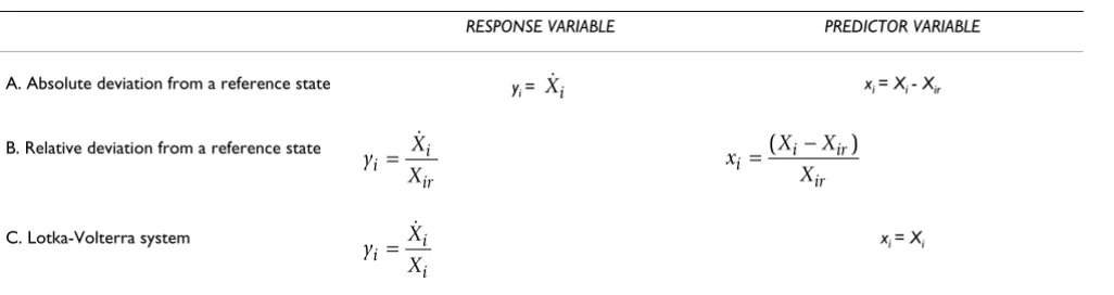
variable is the rate of change of a metabolite, while the predictors are the concentrations of each metabolite in the network. The different linearization models (I-IV) differ in the transformations of the original datasets, which are summarized in Table 1. For example, the response
varia-ble of the linear model in Eq. (4) is given by yi = /Xir, and the predictor variables are transformed as xi = (Xi -Xir)/Xir.
The result of the regression is a matrix of coefficients that indicate to what degree a metabolite Xj affects the
dynam-ics (slope) of another metabolite Xi. In particular, a coef-ficient that is zero or close to zero signals that there is no significant effect of Xj on the slope of Xi. By the same token, a coefficient that is significantly different from zero suggests the presence of an effect, and its value tends to reflect the strength and direction of the interaction. In either case, the coefficients computed from the linear regression provide valuable insight into the connectivity of the network. Furthermore, the estimated coefficients provide constraints on the parameter values of the desired nonlinear model f. Indeed, if f consists of an S-system model, the coefficients estimated from the regression can be converted into combinations of S-system parameters, as is demonstrated in the following theoretical section and illustrated later with a specific example.
Relationships between Estimated Regression Coefficients and S-system Parameters
The regression analysis yields coefficients that offer infor-mation on the connectivity of the network of interest. It also provides clues about the parameter values of the underlying nonlinear network model f in Eq. (1) if this model has the form of an S-system. To determine the rela-tionships between the regression coefficients and the parameters of the S-system, it is convenient to work back-wards by computing the different types of linearizations discussed before for the particular case of S-system mod-els. This derivation is simply a matter of applying Taylor's theorem.
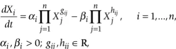
In the S-system formalism, the rate of change in each pool (variable) is represented as the difference between influx into the pool and efflux out of the pool. Each term is approximated by a product of power-law functions, so that the generic form of any S-system model is
Xi
Table 1: Transformation of data for regression analysis
RESPONSE VARIABLE PREDICTOR VARIABLE
A. Absolute deviation from a reference state y
i = xi = Xi - Xir
B. Relative deviation from a reference state
C. Lotka-Volterra system xi = Xi
We assume the general linear model is y = ai0 + Σ(aij xj). The Xi denote experimental time series data for metabolite i, while the slopes ( ) are
estimated from the smooth output functions of the artificial neural network that had been trained on the experimental data. Subscript r denotes the
value of the metabolite at a reference state. Linearization options I and II are included in transformations A and B respectively, assuming that the reference state is a steady state. For a piecewise linear linearization (option III), the data may be transformed following either A or B.
Xi
y X
X
i i
ir
= x X X
X
i i ir
ir
=( − )
y X
X
i i
i =
where n is the number of state variables [13,14]. The expo-nents gij and hij are called kinetic orders and describe the quantitative effect of Xj on the production or degradation of Xi, respectively. A kinetic order of zero implies that the corresponding variable Xj does not have an effect on Xi. If the kinetic order is positive, the effect is activating or aug-menting, and if it is negative, the effect is inhibiting. The multipliers αi and βi are rate constants that quantify the turnover rate of the production or degradation, respectively.
If the Taylor linearization is performed at a steady state, the production term of the S-system model equals the degradation term. The absolute deviation of the first option, zi = Xi - Xis, where the subscript s denotes the value of the variable at steady state, then leads directly to
where
cij = gij - hij,
(cf. [41]). The so-called F-factors Fij are always non-nega-tive, while cij may be either positive or negative depending on the relationship between Xi and Xj. A common scenario is that a variable Xj influences either the production or
degradation of variable Xi, but not both. In this case, a positive (negative) cij implies activation (inhibition) of production or inhibition (activation) of degradation. The special case of cij = 0 permits two possible interpretations: 1) gij = hij = 0, which implies that Xj has no effect on either
production or degradation of Xi; or 2) gij = hij ≠ 0, which means that Xj has the same effect on both production and degradation of Xi. The former case is the more likely, but
there are examples where the latter may be true as well, and this is indeed the case in the small gene network in Figure 1.
Comparing the expression in Eq. (6) with the linear regression results, one sees immediately that each coeffi-cient aij in Eq. (3) corresponds to the product of Fij and cij:
aij = Fijcij. (7)
Thus, once the regression has been performed and the coefficients aij have been estimated, the parameters of the corresponding S-system are constrained – though not fully determined – by Eq. (7). In particular, Eq. (7) does not allow a distinction between various combinations of gij and hij, as long as the two have the same difference. For
dX
dt X X i n
g h i i j g i j h j n j n
i i ij ij
ij ij = − = > ∈ = =
∏
∏
α β α β 1 1 1 0 , ,..., ,, ; , RR,
dz
dt F c z
i
ij ij j j n = =
∑
1 6 , ( )Fij =αiXgsi Xgis Xjsgij− Xnsgin
1 2
1
1 2
Test System
Figure 1
Test System. a) Gene network [42] used as test system for illustrating the proposed methods. Solid arrows represent mate-rial flow, while dashed arrows indicate regulatory signals that either activate (+) or inhibit (-) a process. The network contains two genes, Gene 1 and 2. X1 is the mRNA produced from gene 1, X2 is the enzyme for which the gene codes, and X3 is an inducer protein catalyzed by X2. X4 is the mRNA produced from Gene 2 and X5 is a regulator protein for which the gene
codes. Positive feedback from X3 and negative feedback from X5 are assumed in the production of mRNAs from the two genes.
b) S-system model of the gene network, according to Hlavacek and Savageau [42] and Kikuchi et al. [21].
instance, re-interpreting the regression coefficients as S-system parameters does not differentiate between the overall absence of effect of Xj on Xi (gij = hij = 0) and the same effect of Xj on both the production and degradation of Xi (gij = hij ≠ 0). This observation is related to the obser-vation of Sorribas and Cascante [36] that steady-state measurements are insufficient for completely identifying an S-system model.
Relative deviations from steady state, ui = (Xi - Xis) / Xis, in option II, are assessed in an analogous fashion. In this case one obtains
where
cij = gij - hij,
[41]. Again, the F-factors Fi are positive, while cij may be either positive or negative.
The piecewise linear model for an S-system is easily derived as well. It is given as
where Xjr denotes the value of the variable at the reference state. This case also includes the situation of a single approximation, which however is not necessarily based on a steady-state operating point.
In the case of the Lotka-Volterra linearization, the corre-spondence between computed regression coefficients and S-system parameters is determined most easily by dividing the S-system equations by the corresponding Xi and then linearizing around an operating point. The resulting expressions become especially simple if this point is cho-sen as the steady state. In this case, the relationship between the parameters of the LV system and the S-system are
where cij = gij - hij.
Results
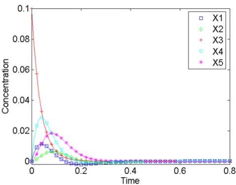
We applied the methods described in the previous sec-tions to simulated time profiles obtained from the small gene network in Figure 1a. Hlavacek and Savageau [42] modeled this network as an S-system with five differential equations (Figure 1b), and Kikuchi et al. [21] used it recently for exploring computational features of their pro-posed structure identification algorithm. The benefit of working with a known model is that complete informa-tion is available about both its structure and parameter values. In particular, it is possible to perform any number of experiments and to produce data and slopes with pre-determined noise levels, which is not typically possible with real data. For this analysis, we thus used simulated noise free "data," which allowed us to skip the neural net-work step of smoothing [23,39].
To generate time profiles, the system was implemented with the parameter values published by Hlavacek and Sav-ageau [42], and as in the analysis of Kikuchi et al. [21], the model was initialized with various perturbations from steady state and numerically integrated over a sufficient time horizon to allow the system to return to the steady state.
Preliminary Analysis
Quasi as a pre-analysis, we examined the guidelines pro-posed by Vance et al. [8]. Indeed, the results show that many of these are applicable to the gene regulatory net-work. The order of the extrema (i.e., the maximum devia-tions from steady state) of the various variables both in time and size is in accordance with their "topological dis-tance" from the perturbed variable, and variables not directly affected by the perturbed variable have zero initial slopes. As an example, the effect of a perturbation in X3 is shown in Figure 2. All variables increase in response, with variables X1 and X4 reaching their maximal deviation from steady state before X2 and X5, suggesting that X1 and X4 precede X2 and X5 in the pathway. The value of the initial slope is different from zero for X1 and X4, implying that these variables are directly affected by X3, whereas X2 and X5 have zero initial slopes suggesting that their responses are mediated through other variables.
Maximal information about the network is obtained when every variable is perturbed sequentially. Experimen-tally, such perturbations could be implemented with modern methods of RNA interference [43] or, for biotech-nological purposes, in a chemostat [9]. In our model case, we can actually identify all kinetic orders that are zero in the original model, and this amounts to determining the connectivity of the pathway. The only relationship this analysis does not pick up is the effect of X2 on X3. This result is not surprising, because the effect of X2 is the same on both the production and degradation of X3, which du
dt F c u
i
i ij j j n = =
∑
( ), ( ) 1 8Fi =αiXgsi Xgis Xisgii− Xnsgin
1 2
1
1 2 ,
dz
dt X X G H u
G g i i jr g i jr h j n j n
ij ij j j n ij i ij ij = − + − = = =
∏
=∏
∑
α β α 1 1 1 ( ) , iij r g r g jr gnrg ij i ij r h
r h
jr h X i X i X ij X in H h X iX i X
1 2
1
1 2
1 2… −… , =β 1 2… iij Xin
nrh
−1
… ,
v
c F i j F X X X X X
ij
ij ijLV ijLV i s
g s g is g js g n
i ii ij
= ≠ =
− −
, , α 11 212… 1… 1…
ss g
ii iLV iLV i s
g s g is g js g nsg in
i ii ij
c F i j F X X X X X
,
, = , =α 11 212… −2… … iin,
leads to cancellation. It is noted that this analysis does not necessarily distinguish between transfer of mass and a positive modulation, because both result in a positive effect on a variable. In a realistic situation, biological knowledge may exclude one of the two options, as in this case, where modulation is the only possibility for the effect of X3 on both X1 and X4, because the former is a pro-tein and the latter are RNA transcripts. For the mathemat-ical model in the S-system form, this is not an issue, as both types of influence are included in the equations in the same way (as a positive kinetic order).
Regression Analysis
While Vance's method works well in this simple noise-free system, it is not scalable to larger and more complex sys-tems. The next step of our analysis is therefore regression according to the four options presented above and with a number of simulated datasets of the gene network that differ in the variable to be perturbed and the size of the perturbation. Because the illustration here uses a known model and artificial data, it is easy to compute the true regression coefficients through differentiation of the S-system model. These coefficients can be used as a
reference for comparisons with coefficients computed from the entire time traces, which mimics the estimation process for (smoothed) actual data.
Options I, II and IV
The results for three of the options (I, II and IV) can be summarized in the following three points, while the piecewise linear model will be discussed afterwards.
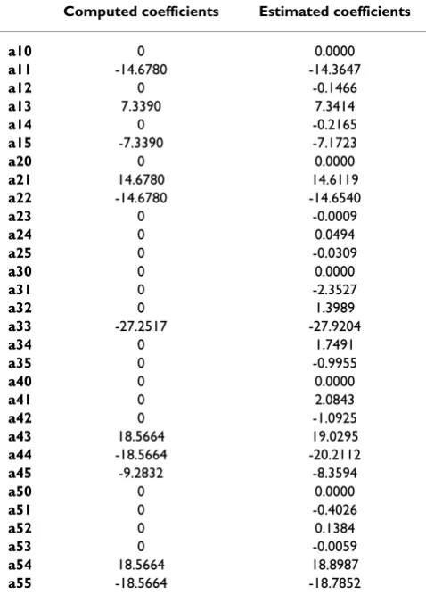
(1) The network connectivity is reflected in the values of the regression coefficients. The values of the estimated coeffi-cients provide strong indication as to which variables have a significant influence on the dynamics of other variables. A comparison between computed and estimated coeffi-cients is shown in Table 2 for the linear model with rela-tive deviations (option II, Eq. 8). Most of the coefficients that in reality are zero (for example a12 and a24) are not estimated as exactly zero, but their values are at least one order of magnitude smaller than the coefficients that are in actuality not zero. Table 2 also indicates that not all coefficients reflect the network correctly. The linear regres-sion gives especially poor estimates for the coefficients associated with variables X3 and X4. A possible explana-tion for X3 is that the effect of X2 is present in the non-lin-ear system, but not in the linnon-lin-ear system, and thus the behavior of X3 must be explained by the other variables. Overall, of the 25 theoretically possible connections, 76% are correctly identified, while 24 % are false positives.
(2) The different linear models give (qualitatively) the same results. A comparison of the results of the three models reveals that the values of the regression coefficients are very similar (see Table 3). The same applies to their signs. Most important, all models correctly identify the connec-tions present in the gene network. They also equally infer the same incorrect relationships. As an example, consider the coefficients associated with X4: all models infer the net positive effect of X3 and the net negative effect of both X4 and X5. At the same time, they also suggest that X1 and X2 have a significant effect on the dynamics of X4. In reality, they do not directly influence X4 (see Figure 1), and it may be that their indirect effect, which is mediated by X3, is causing the false positive result.
(3) The greater the perturbation, the less accurate is the estima-tion of the regression coefficients. The deviation between the estimated and computed coefficients increases as the size of the perturbation increases (see Table 4). For the models obtained by linearizing about the steady state (Eqs. (6) and (8)), this is an expected result, as the Taylor-expan-sion only gives a valid approximation close to steady state. For these systems, "close" may correspond to a perturba-tion of less than 5–10% with respect to the steady-state value. Nonetheless, the greater perturbations still give a relatively good picture in terms of the connectivity of the
Dynamic response of the network after a perturbation in X3 Figure 2
Dynamic response of the network after a perturba-tion in X3 The response is shown as relative deviation from steady state. The guidelines proposed by Vance et al. [8] indi-cate that X1 and X4 precede X2 and X5 because they reach their maximum deviation earlier and the maximal values are larger than those of X2 and X5. All variables respond in a
system. For a 5% perturbation, the fraction of correctly identified connections is 76% and for a two-fold perturba-tion it is still 64 %. Perturbaperturba-tions of more than 5–10 % of the steady state also cause problems for the Lotka-Volterra model, from which one might have expected a higher tol-erance as the linearization is independent of a reference state. It seems that the dynamics of the true system in our particular example is about equally well modeled by the nonlinear LV-model as by the linear models.
Option III
The piecewise linear model was obtained by dividing the whole dataset into three smaller subsets for each variable. The first interval contained the data points from t = 0 to
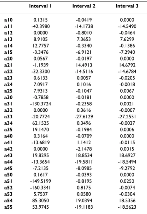
the time of the first extreme value for a given variable (in this case a maximum for all variables). For the perturbed variable (having its first extreme value at t = 0) the first limit point was given by the smallest of the limit points of the other variables. The second interval contained the data points from the first to the second extreme value (a mini-mum), while the third interval included the remaining data points. The midpoint of each interval was taken to be the reference state. The result of the piecewise linear regression for a 5% deviation in X3 is given in Table 5. The first subset does not reflect the interactions of the system especially well, whereas the other two subsets correctly classify 88% and 96%, respectively, of the true connec-tions in the network. It is worth noting that the coeffi-cients associated with X3 in the two last subsets reflect the variable's connectivity to a much greater extent than the other linearization approaches. As the reference state is different from the steady state, the effect of X2 is present in the linear system as well, and thus there is no compensa-tion through the other variables. Another benefit is that the piecewise model tolerates larger perturbations. Even for a two-fold perturbation, the fraction of correctly iden-tified coefficients in the last subset is 84%.
Degree of Similarity as a Measure of Reliability
If we compare the results of all four linearized models, the degree of similarity may provide a measure of how relia-ble the estimated coefficients are, assuming that an inter-action identified in all models is more reliable than an interaction identified in only one or few of the models. Considering the piecewise linear model as three models, yielding a total of 6 models from one dataset, one may thus determine the most likely connectivity for the small gene network. The result is presented in Table 6. Of the 25 possible connections, 12 were identified correctly in all models, either as being positive, negative or non-existent, while an additional 6 connections were correctly identi-fied in either 4 or 5 of the six models. For these six, one of the models misidentifying the type of connection was the first subset of the piecewise linear approximation, which does not reflect the connectivity of the network especially well, as was shown in Table 5. It is also worth noting that only one of the interactions associated with X3 is identi-fied correctly from comparing the six models. The classifi-cation of the remaining four connections varies greatly among the different models, and it is therefore impossible to deduce a type of interaction with sufficient reliability.
Constraining the Parameter Values
In addition to reflecting the connectivity, the coefficients provide likely parameter ranges or likely constraints on parameter values of the true model. As an example, consider variable X1. Table 6 indicates that the variables having a significant effect are X1, X3 and X5. If so, the linear model in Eq. (8) suggests the following:
Table 2: Comparison of computed and estimated coefficients
Computed coefficients Estimated coefficients
a10 0 0.0000
a11 -14.6780 -14.3647
a12 0 -0.1466
a13 7.3390 7.3414
a14 0 -0.2165
a15 -7.3390 -7.1723
a20 0 0.0000
a21 14.6780 14.6119
a22 -14.6780 -14.6540
a23 0 -0.0009
a24 0 0.0494
a25 0 -0.0309
a30 0 0.0000
a31 0 -2.3527
a32 0 1.3989
a33 -27.2517 -27.9204
a34 0 1.7491
a35 0 -0.9955
a40 0 0.0000
a41 0 2.0843
a42 0 -1.0925
a43 18.5664 19.0295
a44 -18.5664 -20.2112
a45 -9.2832 -8.3594
a50 0 0.0000
a51 0 -0.4026
a52 0 0.1384
a53 0 -0.0059
a54 18.5664 18.8987
a55 -18.5664 -18.7852
Regression coefficients for the small gene network (Figure 1), linearized about the steady state and based on relative deviations (option II). The first and second columns contain the computed and estimated regression coefficients, respectively. The regression
coefficients aij refer to the influence of variable j on variable i, while ai0
is the constant term in each regression model. As the table indicates,
the correspondence is good, except for the coefficients relating to X3
and X4 (see Text for explanation). The dataset consisted of 401 data
points in the interval [0,4] and resulted from a simulation in which X3
where and the regression coeffi-cients (aij) are taken from the model in Eq. (4). The values of the variables at steady state are known. Because the kinetic orders may be positive or negative and the cij may result from different combinations of gij's and hij's, it is not possible to deduce directly which exponent is greater than the other. However, in many cases one may have addi-tional information on the system, which further limits the degrees of freedom (e.g., [23]). In addition, the
steady-state equation must be
satisfied and provides yet another constraint.
Discussion
Identifying the structure of metabolic or proteomic net-works from time series is a task that most likely will require large, parallelized computational effort. The search space for the algorithms is typically of high dimen-sion and unknown structure and very often contains numerous local minima. This generic and frequent prob-lem may be ameliorated if the search algorithm is pro-vided with good initial guesses and/or constraints on admissible parameter values. Here, we have shown that linear regression may provide such information directly from the types of data to be expected from future experi-ments. For illustrative purposes, we used artificial data from a known network, but all methods are directly appli-cable to actual profile data and scaleable to large systems.
The coefficients estimated from the different regressions reflect the effect of one variable on another surprisingly well and thus provide a simple fashion of prescreening the
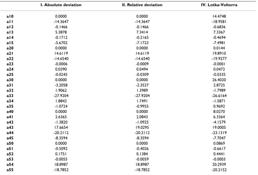
Table 3: Comparison of the different linearization options (I, II and IV)
I. Absolute deviation II. Relative deviation IV. Lotka-Volterra
a10 0.0000 0.0000 14.4748
a11 -14.3647 -14.3647 -18.9581
a12 -0.1466 -0.1466 -0.6836
a13 5.3878 7.3414 7.3367
a14 -0.1712 -0.2165 -0.4694
a15 -5.6702 -7.1723 -7.4981
a20 0.0000 0.0000 0.0144
a21 14.6119 14.6119 19.8910
a22 -14.6540 -14.6540 -19.9277
a23 -0.0006 -0.0009 -0.0001
a24 0.0390 0.0494 0.0472
a25 -0.0245 -0.0309 -0.0335
a30 0.0000 0.0000 26.4020
a31 -3.2058 -2.3527 2.8725
a32 1.9062 1.3989 -1.7989
a33 -27.9204 -27.9204 -26.6164
a34 1.8842 1.7491 -1.5871
a35 -1.0724 -0.9955 0.9692
a40 0.0000 0.0000 8.0270
a41 2.6365 2.0843 6.3364
a42 -1.3820 -1.0925 -4.1579
a43 17.6654 19.0295 19.0005
a44 -20.2112 -20.2112 -23.1319
a45 -8.3594 -8.3594 -7.7047
a50 0.0000 0.0000 0.0869
a51 -0.5092 -0.4026 -0.6617
a52 0.1751 0.1384 0.4441
a53 -0.0055 -0.0059 -0.0003
a54 18.8987 18.8987 20.2939
a55 -18.7852 -18.7852 -20.2152
Estimated coefficients for three of the linearization approaches: absolute deviation from steady state (left column), relative deviation from steady state (center column) and Lotka-Volterra linearization (right column). The dataset consisted of 401 data points in the interval [0,4] and resulted
from a simulation in which X3 was perturbed at t = 0 to a value 5% above its steady-state value.
F c a
F c a
F c a
c g h
c g h
1 11 11
1 13 13
1 15 15
11 11 11
13 13 13
0 0 ≈
≈ ≈
= − < = − > ,
, ,
, , cc15 =g15−h15<0.
F1=α1 1Xg11s −1X3g13s X5g15s
α1 1X 11s X313X515 β1 1X 11X313X515
g s g
s g
s h
s h
connectivity of the network. In addition, the estimated coefficients provide constraints on the parameter values, if the alleged nonlinear model has the form of an S-system. To explore the pre-assessment of data as fully as feasible, we studied four linearization strategies: using an absolute deviation from steady state; a relative deviation from steady state; piecewise linearization; and Lotka-Volterra linearization. Interestingly, all models gave qualitatively similar results for the analyzed example, and this degree of similarity may provide a measure of how reliable the identified connections are. Specifically, of the 25 possible connections in the small gene network studied, 19 were identified correctly in at least 83 % of the regression analyses.
Table 4: The effect of the size of the perturbation
Computed 5 % 10 % 50 % 200 %
a10 0 0.0000 0.0000 0.0001 0.0008
a11 -14.6780 -14.3647 -14.1817 -13.1496 -11.3439
a12 0 -0.1466 -0.1429 -0.0671 0.5735
a13 7.3390 7.3414 7.3438 7.3598 7.3735
a14 0 -0.2165 -0.3673 -1.2462 -2.7619
a15 -7.3390 -7.1723 -7.0780 -6.4846 -5.2501
a20 0 0.0000 0.0000 0.0000 -0.0003
a21 14.6780 14.6119 14.5748 14.4207 14.5029
a22 -14.6780 -14.6540 -14.6623 -14.7503 -15.1862
a23 0 -0.0009 -0.0016 -0.0054 -0.0070
a24 0 0.0494 0.0839 0.2494 0.3462
a25 0 -0.0309 -0.0464 -0.1119 -0.0951
a30 0 0.0000 0.0000 0.0004 0.0038
a31 0 -2.3527 -4.5412 -18.2307 -46.8953
a32 0 1.3989 2.6336 9.8422 24.4004
a33 -27.2517 -27.9204 -28.5955 -34.0204 -54.4047
a34 0 1.7491 3.4009 14.0961 39.3252
a35 0 -0.9955 -1.8949 -7.0627 -15.4759
a40 0 0.0000 0.0000 -0.0001 0.0001
a41 0 2.0843 3.7814 14.7316 41.5863
a42 0 -1.0925 -1.7693 -5.5766 -13.2688
a43 18.5664 19.0295 19.4964 23.2397 37.1866
a44 -18.5664 -20.2112 -21.6608 -31.4631 -58.1065
a45 -9.2832 -8.3594 -7.6404 -3.2226 6.5808
a50 0 0.0000 0.0000 -0.0001 -0.0015
a51 0 -0.4026 -0.6581 -2.5848 -10.1097
a52 0 0.1384 0.0830 -0.1317 0.1582
a53 0 -0.0059 -0.0110 -0.0435 -0.0879
a54 18.5664 18.8987 19.1602 21.0620 27.2722
a55 -18.5664 -18.7852 -18.9201 -20.0013 -24.0836
Overall, the estimated coefficients deviate more strongly from the corresponding computed values as the perturbation increases. However, there are substantial differences between variables. The
coefficients associated with variable X2, for example, are hardly
influenced, while the coefficients associated with X3 are strongly
affected. Overall, the method seems to produce the best results for perturbation up to 10%. The datasets for the regression consisted of 401 data points in the interval [0,4] and the method of linearization was option II.
Table 5: Results for piecewise linear regression
Interval 1 Interval 2 Interval 3
a10 0.1315 -0.0419 0.0000
a11 -42.3980 -14.1738 -14.5490
a12 0.0000 -0.8010 -0.0464
a13 8.9105 7.3653 7.6299
a14 12.7757 -0.3340 -0.1386
a15 -3.3476 -6.9121 -7.2940
a20 0.0567 -0.0197 0.0000
a21 -1.1939 14.4913 14.6792
a22 -32.3300 -14.5116 -14.6784
a23 0.6133 0.0057 -0.0205
a24 7.0917 0.1016 -0.0018
a25 7.9313 -0.1047 0.0067
a30 -0.7858 -0.0181 0.0000
a31 -130.3724 -0.2358 0.0021
a32 0.0000 0.3616 -0.0007
a33 -20.7724 -27.6129 -27.2551
a34 62.1525 0.3496 -0.0027
a35 19.1470 -0.1984 0.0006
a40 0.3164 -0.0709 0.0000
a41 -13.6819 1.1412 -0.0115
a42 0.0000 -2.1478 0.0015
a43 19.8295 18.8534 18.6927
a44 -13.3654 -19.5811 -18.5494
a45 -7.2135 -8.0985 -9.2792
a50 0.1617 -0.0393 0.0000
a51 -149.5199 -0.8195 0.0250
a52 -160.3341 0.8175 -0.0074
a53 5.7537 0.0580 -0.0304
a54 85.3050 19.0394 18.5356
a55 53.9745 -19.1183 -18.5623
The complete dataset is divided into three subsets for each variable, where the first and second extreme values serve as breakpoints. The datasets for the regression consisted of 401 data points in the interval
[0,4] and resulted from a simulation in which X3 was perturbed at t =
0 to a value 5% above its steady-state value.
Table 6: Collective inference of the gene network based on results from all linearizations
X1 X2 X3 X4 X5
X1 - (100 %) 0 (67 %) + (100 %) 0 (83 %) - (100 %)
X2 + (100 %) - (100 %) 0 (100 %) 0 (83 %) 0 (83 %)
X3 ? ? - (100 %) ? ?
X4 + (67 %) - (67 %) + (100 %) - (100 %) - (100%)
X5 - (83 %) 0 (83 %) 0 (83 %) + (100 %) - (100 %)
A concern of any linearization approach is the validity of the linear approximation. However, as long as the pertur-bation from steady state remains relatively small, the esti-mated linear model is likely to be a good fit of the actual nonlinear model, at least qualitatively. This limitation may furthermore be alleviated by fitting the profile data in a piecewise linear fashion. As most reference states in this case are different from the steady state, this strategy has the added benefit that more of the true relationships within the nonlinear model are likely to be preserved. As an alternative, one could explore the performance of the so-called "log-linear" model, which is linear in log-trans-formed variables [44].
The Lotka-Volterra linearization did not perform as well as expected with regard to large perturbations. This may be a consequence of the particular example, which was originally in S-system form rather than in a form more conducive to the LV structure, which emphasizes interac-tions between pairs of variables. Since it is easy to perform the LV analysis along with the other regressions discussed here, it may be advisable to execute all four analyses.
The illustrative model used for testing the procedure con-sisted of a relatively small system with only five variables and relatively few interactions. Nonetheless, one should recall that this very system required substantial identifica-tion time in a direct estimaidentifica-tion approach [21]. In order to check how scaleable the results of the proposed lineariza-tion method are, the method should be tested on larger systems. Some preliminary analyses suggest that the method works well, but that the likelihood of misidenti-fied connections may grow with the size of the system, as one might expect. At the same time, experience with actual biological networks, for instance in ecology and metabo-lism, suggests that larger systems are often more robust in a sense that they do not deviate as much from the steady state as smaller systems. If this trend holds in general, the linearization becomes a more accurate representation as larger networks are being investigated and the proposed methods will therefore yield more reliable initial indicators of network connectivity. Independent of these issues, the methods proposed here will very likely be more valuable for bigger systems than other methods that are presently available, because without some preprocessing of the data and effectively priming the search, as it is pro-posed here, the combinatorial explosion will most cer-tainly gain the upper hand eventually.
Competing interests
None declared.Authors' contributions
SRV performed the analysis and prepared the results. JS developed and implemented the neural network for
computation of slopes. EOV developed the basic ideas and directed the project.
Appendix
It was recently shown that good parameter estimates of S-system models from metabolic profiles might be obtained by training an artificial neural network (ANN) directly with the experimental data. The result of this training is a so-called universal function which smoothes the data with predetermined precision and also allows the straightforward computation of slopes that can be used for network identification purposes. This appendix briefly outlines the procedure; details can be found in Almeida [45] and Voit and Almeida [24]. The ANN consists of three layers; one input layer, one hidden layer and one output layer. The input layer consists of the measurement time points, the hidden layer has no direct biological interpretation, and the output layer contains the metabo-lite concentrations or levels of protein expression that the ANN is being trained to represent. The node values of the ANN in the hidden layer are calculated from a linear com-bination of input values with different weights according to a multivariate logistic equation. Similarly, the values of the output layer are determined from linear combinations of the hidden node values with different weights, again using a multivariate logistic function. It is known that this type of nested multivariate logistic function has unlimited flexibility in modeling nonlinearities [46].
Noise and sample size do not have a devastating effect on the results of the ANN-method, as long as the true trend is well represented [39]. In fact, the ANN approach provides an unlimited number of sampling points, as values at any desired time points may be estimated from the universal output function. Finally, the calculation of the slopes of the smooth output functions is mathematically unwieldy, but computationally straightforward.
The use of the entire time course is in stark contrast to ear-lier methods of parameter estimation and structure iden-tification in metabolic networks. Mendes and Kell [37] applied their ANN-based parameter estimation to steady-state data, while we are using time profiles.
Chevalier and co-workers [32] first fitted the nonlinear solution with a linear model (as shown in Eq. 3), expressed this solution in terms of eigenvectors and eigen-values, and then obtained the slopes by numerical differ-entiation. Sorribas et al. [47] suggested a variation on this approach, based on discretizing the solution of Eq. (3) as
z(tk + 1) = z(tk)exp(h·A), (A1)
exp(h·A) is the output. Instead of estimating the slopes, they obtain the Jacobian directly by
expanded in its Taylor-series. This approach yields a faster convergence to the elements of the Jacobian than the one suggested by Chevalier et al. [32], but the regression of Eq. (A1) is very sensitive to noise and missing data points.
Our approach takes advantage of the entire time course and is therefore less sensitive to the particularities of assessing a system at a single point. The ANN itself does not provide much insight, because it is strictly a black-box model, but it is a valuable tool for controlling problems that are germane to any data analysis, namely noise, meas-urement inaccuracies, and missing data.
Acknowledgments
This research was carried out during S.R.V.'s scientific visit at the Medical University of South Carolina. The work was supported by a Quantitative Systems Biotechnology grant (BES-0120288; E.O. Voit, PI) from the National Science Foundation, a National Heart, Lung and Blood Institute Proteomics Initiative through contract N01-HV-28181 (D. Knapp, PI), and an Interdisciplinary USC/MUSC grant (E.P. Gatzke, PI). Any opinions, find-ings, and conclusions or recommendations expressed in this material are those of the authors and do not necessarily reflect the views of the spon-soring institutions.
References
1. Goodenowe D: Metabolic network analysis: Integrating com-prehensive genomic and metabolomic data to understand development and disease (abstract). Chapel Hill, NC; 2001. 2. Goodenowe D: Metabolomic analysis with fourier transform
ion cyclotron resonance mass spectrometry.Metabolic Profiling: Its role in Biomarker Discovery and Gene Function Analysis Edited by: GoodacreR and HarriganGG. Dordrecht, The Netherlands, Kluwer Academic Publishing; 2003:125-139.
3. Neves AR, Ventura R, Mansour N, Shearman C, Gasson MJ, Maycook C, Ramos A, Santos H: Is the glycolytic flux in Lactococcus lactis primarily controlled by the redox charge? J Biol Chem 2002,
277:28088-28098.
4. Szyperski T: 13C-NMR, MS and metabolic flux balancing in biotechnology research.Quart Rev Biophys 1998, 31:41-106. 5. Gerner C, Vejda S, Gelbmann D, Bayer E, Gotzman J,
Schulte-Her-mann R, Mikulits W: Concomitant determination of absolute values of cellular protein amounts,synthesis rates, and
turn-over rates by quantitative proteome profiling. Mol Cell
Proteomics 2002, 1:528-537.
6. Mckenzie JA, Strauss PR: A quantitative method for measuring protein phosphorylation.Anal Biochem 2003, 313:9-16.
7. Alizadeh AA, Ross DT, Perou CM, van de Rijn M: Towards a novel classification of human malignancies based on gene expres-sion pattern.J Pathol 2001, 195:41-52.
8. Vance W, Arkin AP, Ross J: Determination of causal connectiv-ities of species in reaction networks.Proc Natl Acad Sci U S A
2002, 99:5816-5821.
9. Torralba AS, Yu K, Shen P, Oefner PJ, Ross J: Experimental test of a method for determining causal connectivities of species in reactions.Proc Natl Acad Sci U S A 2003, 100:1494-1498.
10. Samoilov M, Arkin AP, Ross J: On the deduction of chemical reaction pathways from measurements of time-series of concentrations.Chaos 2001, 11:108-114.
11. Peschel M, Mende W: The predator-prey model: Do we live in a Volterra world? Berlin, Akademie-Verlag; 1986.
12. Hernández-Bermejo B, Fairén V: Lotka-Volterra representation of general nonlinear systems.Math Biosci 1997, 140:1-32.
13. Savageau MA: Biochemical systems analysis. 1. Some mathe-matical properties of the rate law for the component enzy-matic reactions.J Theor Biol 1969, 25:365-369.
14. Savageau MA: Biochemical systems analysis. 2. The steady-state solutions for an n-pool system using a power law approximation.J Theor Biol 1969, 25:370-379.
15. Voit EO: Computational analysis of biochemical systems: a practical guide for biochemists and molecular biologists Cambridge, Cambridge Univer-sity Press; 2000-531 s..
16. Voit EO, Savageau MA: Power-law approach to modeling bio-logical systems; II. Application to ethanol production.J Fer-ment Technol 1982, 60:229-232.
17. Voit EO, Savageau MA: Power-law approach to modeling bio-logical systems; III. Methods of analysis.J Ferment Technol 1982,
60:233-241.
18. Akutsu T, Miyano S, Kuhara S: Inferring qualitative relations in genetic networks and metabolic pathways.Bioinformatics 2000,
16:727-734.
19. Sakamoto E, Iba H: Inferring a system of differential equations for a gene regulatory network by using genetic programming. Proc of the 2001 Congr Evolut Comput CEC2001
2001:720-726.
20. Maki Y, Tominaga D, Okamoto M, Watanabe S, Eguchi Y: Develop-ment of a system for the inference of large scale genetic networks.Pac Symp Biocomput 2001:446-458.
21. Kikuchi S, Tominaga D, Arita M, Takahashi K, Tomita M: Dynamic modeling of genetic networks using genetic algorithm and S-system.Bioinformatics 2003, 19:643-650.
22. Voit EO, Almeida J: Dynamic profiling and canonical modeling: Powerful partners in metabolic pathway identification. Meta-bolic Profiling: Its role in Biomarker Discovery and Gene Function Analysis
Edited by: GoodacreR and HarriganGG. Dordrect, The Netherlands, Kluwer Academic Publishing; 2003:125-139.
23. Almeida J, Voit EO: Neural-network-based parameter estima-tion in complex biomedical systems.Genome Informatics 2003,
14:114-123.
24. Voit EO, Almeida J: Decoupling dynamical systems for pathway identification from metabolic profiles. Bioinformatics 2004,
20:1670-1681.
25. Karnaukhov AV, Karnaukhova EV: Application of a new method of nonlinear dynamical system identification to biochemical problems.Biochemistry (Mosc) 2003, 68:253-259.
26. Godfrey KR, Chapman MJ, Vajda S: Identifiability and indistin-guishability of nonlinear pharmacokinetic models.J Pharma-cokinet Biopharm 1994, 22:229-257.
27. Friedman N, Linial M, Nachman I, Pe'er D: Using Bayesian net-works to analyze expression data.J Comput Biol 2000, 7:601-620. 28. Arkin AP, Shen PD, Ross J: A test case of correlation metric con-struction of a reaction pathway from measurements.Science
1997, 277:1275-1279.
29. Butte AJ, Kohane IS: Mutual information relevance networks: functional genomic clustering using pairwise entropy measurements.Pac Symp Biocomput 2000:418-429.
30. Kikuchi S, Tominaga D, Arita M, Tomita M: Pathway finding from
given time courses using genetic algorithms. Genome
Informatics 2001, 12:304-305.
31. D'Haeseleer P, Wen X, Fuhrman S, Somogyi R: Linear modeling of mRNA expression levels during CNS development and injury.Pac Symp Biocomput 1999:41-52.
32. Chevalier T, Schreiber I, Ross J: Toward a systematic
determina-tion of complex reacdetermina-tion mechanisms. J Phys Chem 1993,
97:6776-6787.
33. Diaz-Sierra R, Fairén V: Simplified method for the computation of parameters of power-law rate equations from time-series.
Math Biosci 2001, 171:1-19.
34. Diaz-Sierra R, Lozano JB, Fairén V: Deduction of chemical mech-anisms from the linear response around steady state.J Phys Chem 1999, 103:337-343.
35. Gardner Timothy S., di Bernardo Diego, Lorenz David, Collins James J.: Inferring Genetic Networks and Identifying Compound
Mode of Action via Expression Profiling. Science 2003,
301:102-105.
36. Sorribas A, Cascante M: Structure Identifiability in Metabolic Pathways - Parameter- Estimation in Models Based on the Power-Law Formalism.Biochem J 1994, 298:303-311.
Publish with BioMed Central and every scientist can read your work free of charge
"BioMed Central will be the most significant development for disseminating the results of biomedical researc h in our lifetime."
Sir Paul Nurse, Cancer Research UK
Your research papers will be:
available free of charge to the entire biomedical community
peer reviewed and published immediately upon acceptance
cited in PubMed and archived on PubMed Central
yours — you keep the copyright
Submit your manuscript here:
http://www.biomedcentral.com/info/publishing_adv.asp
BioMedcentral 37. Mendes P, Kell DB: On the analysis of the inverse problem of
metabolic pathways using artificial neural networks. Biosys-tems 1996, 38:15-28.
38. Chen L, Bernard O, Bastin G, Angelov P: Hybrid modeling of bio-technological processes using neural networks. Control Eng Pract 2000, 8:821-827.
39. Voit EO, Almeida JS: Decoupling dynamical systems for path-way identification.Bioinformatics 2004, 20:1670-1681.
40. Voit EO, Savageau MA: Equivalence between S-systems and Volterra-systems.Math Biosci 1986, 78:47-55.
41. Savageau MA: Biochemical systems analysis: a study of function and design in molecular biology Reading, Mass., Addison-Wesley; 1976-379 s.. 42. Hlavacek WS, Savageau MA: Rules for coupled expression of
reg-ulator and effector genes in inducible circuits.J Mol Biol 1996,
255:121-139.
43. Dykxhoorn DM, Novina CD, Sharp PA: Killing the messenger: Short RNAs that silence gene expression.Nat Rev Mol Cell Biol
2003, 4:457-467.
44. Hatzimanikatis V, Bailey JE: MCA has more to say.J Theor Biol 1996,
182:233-242.
45. Almeida J: Predictive non-linear modeling of complex data by artificial neural networks.Curr Opin Biotechnol 2002, 13:72-76. 46. Funahashi K,I,: On the approximate realization of continuous
mappings by neural networks.Neural Networks 1989, 2:183-192. 47. Sorribas A, Lozano JB, Fairén V: Deriving chemical and biochem-ical model networks from experimental measurements.