The GRAPE aerosol retrieval algorithm

(1)

Atmos. Meas. Tech., 2, 679–701, 2009 www.atmos-meas-tech.net/2/679/2009/

Atmospheric

Measurement

Techniques

The GRAPE aerosol retrieval algorithm

G. E. Thomas1, C. A. Poulsen2, A. M. Sayer1, S. H. Marsh1,*, S. M. Dean1,**, E. Carboni1, R. Siddans2, R. G. Grainger1, and B. N. Lawrence2

1_{Atmospheric, Oceanic and Planetary Physics, University of Oxford, Oxford, UK}

2_{Space Science and Technology Department, Rutherford Appleton Laboratory, Chilton, Didcot, UK} *_{present address: Department of Medical Physics and Bioengineering, Christchurch Hospital, New Zealand} **_{present address: National Institute of Water and Atmospheric Research, Wellington, New Zealand} Received: 12 March 2009 – Published in Atmos. Meas. Tech. Discuss.: 8 April 2009

Revised: 22 October 2009 – Accepted: 23 October 2009 – Published: 6 November 2009

Abstract. The aerosol component of the Oxford-Rutherford Aerosol and Cloud (ORAC) combined cloud and aerosol re-trieval scheme is described and the theoretical performance of the algorithm is analysed. ORAC is an optimal estima-tion retrieval scheme for deriving cloud and aerosol proper-ties from measurements made by imaging satellite radiome-ters and, when applied to cloud free radiances, provides esti-mates of aerosol optical depth at a wavelength of 550 nm, aerosol effective radius and surface reflectance at 550 nm. The aerosol retrieval component of ORAC has several in-carnations – this paper addresses the version which operates in conjunction with the cloud retrieval component of ORAC (described by Watts et al., 1998), as applied in producing the Global Retrieval of ATSR Cloud Parameters and Evaluation (GRAPE) data-set.

The algorithm is described in detail and its performance examined. This includes a discussion of errors resulting from the formulation of the forward model, sensitivity of the retrieval to the measurements and a priori constraints, and errors resulting from assumptions made about the atmo-spheric/surface state.

1 Introduction

Despite the important role that atmospheric aerosols play in both climate forcing (both direct and through their inter-actions with clouds) (IPCC, 2007; Lohmann and Feichter, 2005) and air quality, there are relatively few long term data sets showing their spatial distribution and evolution through time. Imaging satellite instruments offer the abil-ity to provide such measurements and many algorithms have been developed to exploit this ability for specific instruments

Correspondence to: G. E. Thomas ([email protected])

(Veefkind and de Leeuw, 1998; Mishchenko et al., 1999; Martonchik et al., 1998, 2002; von Hoyningen-Huene et al., 2003; Remer et al., 2005; Grey et al., 2006). In this paper an optimal estimation algorithm for the retrieval of aerosol loading from space-borne visible/near-infrared radiometers, is described and an indepth characterisation of its theoretical performance when applied to nadir-view measurements from the Along Track Scanning Radiometer 2 (ATSR-2) is given.

The retrieval of aerosol properties from satellite radiome-ters is a challanging problem for three main reasons:

1. Aerosol retrievals are highly sensitive to cloud contami-nation. The much greater particle size and optical thick-ness of clouds compared to background aerosol means that even a small amount of cloud contamination will greatly effect the retrieved aerosol properties.

2. It is difficult to disentangle the top-of-atmosphere (TOA) radiance contribution of aerosol from the sur-face contribution. This is particularly true over bright and heterogeneous land surfaces, where the TOA signal can dominated by the surface.

3. Even taking the above two factors as read, there are still many more factors effecting the TOA signal than cur-rent measurement systems can unambiguously distin-guish. These factors include the gaseous composition of the atmosphere as well as properties of the aerosol it-self (composition, variation with height, particle shape, mixing state, etc.)

In order to overcome these problems, a number of differ-ent approaches to aerosol retrieval from satellite radiometers have been developed. All of these algorithms rely on emper-ical thresholds of the measured radiance (be it magnitude, ra-tios at different wavelengths or spatial variability) to remove cloudy pixels (Ackerman et al., 1998; G´omez-Chova et al., 2007; Birks, 2007). The main parameter retrieved by most

(2)

680 G. E. Thomas et al.: Aerosol retrieval algorithm algorithms is the aerosol optical depth (AOD) at some

mea-surement wavelength. Many also use the spectral variance of the AOD to give an indication of the size and composition of aerosols by using a range of representative aerosol types or mixtures of components (for which the size and compo-sition is fixed) and picking the one that best reproduces the observed radiance.

Perhaps the biggest difference in the various algorithms is in how they separate the surface and atmospheric contri-butions to TOA signal. The approach taken is largely de-termined by the capabilities of the instrument being used. Where the instrument has relatively high spectral resolution, such as the MODerate resolution Imaging Spectroradiometer (MODIS) or the MEdium Resolution Imaging Spectrometer (MERIS), so called dark-target algorithms are used. These use an assumption of either the surface reflectance, or the extinction coefficient of aerosol, being effectively zero at a given wavelength. Using this assumption the AOD, or sur-face reflectance (depending on which assumption is used), can be unambiguously defined, allowing the optical depth and surface reflectance to be derived at different wavelengths on the basis of assumed aerosol properties and a model of the spectral reflectance of the surface. For example, the stan-dard MODIS aerosol product makes use of both of these approaches. Over the ocean (Remer et al., 2005) the as-sumption is made that the surface reflectance at wavelengths greater than 0.66µm is zero, thus allowing the clear sky TOA signal at such wavelengths to be entirely modelled as a prod-uct of aerosol and Rayleigh scattering, plus absorption. A predefined set of bimodal aerosol models can thus be fit-ted to the observed radiance in 6 channels, incorporating a model of the ocean reflectance for shorter wavelength chan-nels, by varying the mixing ratio between the two modes. The retrieval thus gives the AOD, the ratio between the fine and coarse modes of the aerosol distribution and, by pick-ing the best fittpick-ing of the 20 fine and course mode combi-nations, an indication of aerosol type. This basic approach is commonly used for aerosol retrievals over ocean by many other algorithms and instruments including MERIS (Antoine and Morel, 1999), ATSR (Veefkind and de Leeuw, 1998), AVHRR (Mishchenko et al., 1999).

Over land MODIS (Levy et al., 2007) uses the approxima-tion that the AOD at 2.12µm is close to zero, and thus the TOA signal is dominated by the surface contribution. This, along with assumptions of about the spectral variation of the reflectance of vegitated surfaces, the so called dark-dense ve-gitation (DDV) approximation, allows the AOD to be esti-mated from measuresments at shorter wavelengths. MERIS also uses a DDV approach over land (Santer et al., 1999), al-though it lacks channels in the infrared, so has to rely solely on constraints on the spectral shape of the surface.

If measurements of the same air mass are available from different viewing geometries it is possible to add angular constraints to the retrieval of aerosol. The main instru-ments which provide such multi-angle measurinstru-ments are the

Multi-angle Imaging Spectro-Radiometer (MISR), on board NASA’s terra platfrom, and the ATSR series of instruments launched on ESA satellites. Both instruments not only pro-vide measurements in the nadir direction but also viewing at an angle along the orbital track of the instrument. Due to the high orbital velocity of low Earth orbit satellites, such instru-ments thereby provide multiple measureinstru-ments of the same surface point at different viewing zenith angles, separated by only a few tens of seconds. ATSR provides two views, one in the nadir and one centred at 55◦along the orbital track, while MISR provides a total of nine views with maximum viewing zenith angles of approximately±70◦. Over land, such mea-surements allow the separation of the atmospheric contribu-tion to the TOA radiance from that from the surface because the ratio of the surface reflectance at different viewing ge-ometries shows little angular dependance, since the size of the surface scattering elements are so much larger than the wavelengths being used (Flowerdew and Haigh, 1995). The simplest approach is to assume that this ratio is in fact con-stant with respect to wavelength, as is used by Veefkind and de Leeuw (1998) for ATSR retrievals. North (2002) shows how it is also possible to use the angular constraint to fit a simple empirical surface BRDF model to ATSR measure-ments, providing a retrieval of spectral surface reflectance. In both approaches, the atmospheric path radiance for each instrument channel and view is fitted using a range of aerosol types, thus providing an estimate of the AOD.

This angular constraint approach is also used in MISR re-trievals (Dinner et al., 2005), but only as a first step in reduc-ing the number of aerosol types made available to a second retrieval, based on a different assumption. In this second ap-proach, described by Martonchik et al. (1998), the clear-sky atmosphere is assumed to be homogenous over a region of 17.6×17.6 km (containing 256 individual MISR pixels). Un-der the assumption that the atmospheric and surface signals are additive, a spatial scatter matrix can be constructed that doesn’t depend on the atmospheric path radiance, by express-ing the signal in each pixel as a bias relative to some refer-ence pixel within the retrieval area. The TOA radiance for each pixel can then be reconstructed using a principal com-ponent decomposition of this matrix and an atmospheric path radiance calculated using a range of aerosol types.

The ORAC algorithm is somewhat different than the al-gorithms described above, in that it is not built around any particular method of separating the surface and atmospheric contributions to the TOA signal. Rather it makes use of an optimal estimation retrieval scheme to fit modelled radiances across a series of wavelength bands (channels) to radiances measured by a satellite instrument, as a function of aerosol optical depth, effective radius and surface reflectance, sub-ject to constraint by a priori knowledge of these parame-ters. The algorithm was developed from the Enhanced Cloud Processor (ECP) (Watts et al., 1998) and the version de-scribed here is part of a unified cloud and aerosol algorithm. This algorithm uses a empirical cloud flagging scheme to

(3)

G. E. Thomas et al.: Aerosol retrieval algorithm 681 differentiate cloud and aerosol pixels. Pixels identified as

cloud have the cloud retrieval algorithm applied, with the re-maining pixels having the aerosol retrieval applied.The al-gorithm has been applied to ATSR-2, Advanced-ATSR and Spinning Enhanced Visible-InfraRed Imager (SEVIRI) data (Kokhanovsky et al., 2007; Thomas et al., 2007b), including the creation of the GRAPE global cloud and aerosol data-set derived from the full ATSR-2 data-data-set, spanning 1995– 20011. For descriptions of the ATSR-2, AATSR and SEVIRI instruments the reader is referred to Mutlow et al. (1999), Llewellyn-Jones et al. (2001) and Aminou et al. (1997), re-spectively.

It is important to emphasize that this version of the algo-rithm, hence referred to as the GRAPE algorithm to distin-guish it from the wider family of algorithms which carry the name ORAC, is primarily a cloud retrieval. The inclusion of a simple aerosol retrieval can be considered a way of adding value to the GRAPE cloud products and does not represent the state-of-the-art ORAC aerosol retrieval. There currently exist two further versions of the ORAC aerosol algorihm, which are more advanced stand alone aerosol retrievals. The GRAPE algorithm uses a relatively simple forward model, particularly in its treatment of the surface reflectance, which (in common with the cloud retrieval) is treated as Lamber-tian, and in its treatment of different aerosol types. This re-sults in important limitations to the algorithm:

– The algorithm is only applicable over surfaces which can be reasonably approximated by a Lambertian re-flectance, such as the ocean surface far from the sunglint region, and homogeneous land surfaces.

– The use of a Lambertian surface reflectance prohibits the inclusion of near simultaneous observations of the same scene at different viewing geometries, such as offered by the ATSR instruments’ dual-view system. Even if a surface can be approximated with an effec-tive Lambertain reflectance for a given viewing geom-etry, this value can be different for different viewing geometries.

– In the case of instruments such as ATSR-2 and SE-VIRI, which have a small number of channels in the visible and near-infrared, the retrieval becomes highly dependant on good a priori knowledge of the surface reflectance. This is because the measurements do not contain enough information to decouple the surface and atmospheric components of the signal.

Despite these limitations, the GRAPE dataset has shown that the algorithm can provide aerosol properties of suffient 1_{GRAPE was a UK Natural Environment Research Council} project. The full GRAPE data-set is freely available for download from the British Atmospheric Data Centre. See http://badc.nerc.ac. uk/data/grape/ for further details.

accuracy (i.e. with a random error of _.0.1) to be scien-tifically interesting, particularly over the open ocean, and has been applied in the study of aerosol cloud interactions (Bulgin et al., 2008; Quaas et al., 2009). A validation of the GRAPE oceanic AODs against ocean and coastal AERONET sites, and comparisons with the Global Aerosol Climatology Project (GACP) AOD product derived from Advanced Very High Resolution Radiometer measurements, is presented by Thomas et al. (2009b). This study finds a correlation of 0.79 between the AERONET and GRAPE AODs over ocean pix-els, with a best fit line of τG=(0.08±0.04)+(1.0±0.1)τA, whereτG andτA are the 550 nm AODs from GRAPE and AERONET, respectively. Over land pixels, however, the GRAPE product AOD product has been found to be very noisey and has thus not been validated. The 0.08 offset in GRAPE oceanic AODs when compared to AERONET mea-surements could be partially due to the coastal location of most of the AERONET sites, as the ocean surface model used to set the a priori is most accurate when applied to the deep ocean. For an overview of all versions of the ORAC aerosol algorithm, including a multiview algorithm that makes use of a BRDF description of the surface reflectance, the reader is referred to Thomas et al. (2009a).

In Sect. 2 the ORAC forward model and numerical re-trieval scheme are described. Sect. 3 is devoted to a dis-cussion of the algorithm’s performance and limitations, in-cluding the sensitivity of the algorithm and investigation of sources of error. The results are summarised and conclusions drawn from them in Sect. 4.

2 Forward model and retrieval algorithm

2.1 The forward model

The GRAPE algorithm aerosol forward model can be thought of as being composed of four components:

1. A model of aerosol radiative properties (single scat-ter albedo, extinction coefficient and phase function) at the required wavelengths as a function of aerosol size distribution and spectral refractive indices. Ide-ally the aerosol radiative properties should be computed across the channel bandpass functions of the instrument in question, but for most radiometers the width of each channel is small compared to the scale over which the aerosol radiative properties vary and thus the computa-tion can be done for the weighted centre wavelength of each channel.

2. A model of gas absorption (or emission) over the band-pass of each channel.

3. A model or measurements of the surface reflectance, both of the land and ocean.

(4)

682 G. E. Thomas et al.: Aerosol retrieval algorithm 4. A radiative transfer model, which predicts the top of

at-mosphere radiance as a function of the radiative proper-ties produced by the aerosol and gas models, the surface reflectance, and illumination and viewing angle. For reasons of numerical efficiency, radiative transfer cal-culations are done off-line for a range of aerosol properties and viewing geometries to produce look-up tables, which are then used to predict the radiance during retrieval runs. The GRAPE algorithm uses Mie scattering to relate aerosol mi-crophysical properties to their radiative properties. It should be noted that Mie scattering is only applicable to spherical particles and thus its use will introduce errors in the radia-tive properties of non-spherical aerosol particles (the most notable example being mineral dust). Although not included in this analysis, the development of non-spherical scattering code for use with the ORAC scheme is underway.

Microphysical properties are taken from published de-scriptions of typical atmospheric aerosol types, such as those found in the Optical Properties of Aerosols and Clouds (OPAC) database (Hess et al., 1998). Such models typi-cally describe a range of atmospheric aerosol classes, each of which is made up of an external mixture of multiple com-ponents of a given refractive index, size distribution and mix-ing ratio. In external mixtures each component is assumed to exist separately from the others, with its own size distribu-tion. For use with the GRAPE algorithm, each component is assumed to have a log-normal size distribution

n(r)=√N0 2π

1 lnS

1 rexp

"

−(lnr−lnrm) 2 2ln2S

#

(1) where the median radiusrmand spreadS(where the

stan-dard deviation of lnr is lnS) are taken from the aerosol database.

Mie scattering theory is then used to produce the single scattering albedo (ωi), extinction coefficient (β_iext) and phase

function (pi) of each component,i, from which the values

for the complete aerosol class can be calculated using: βext=

6iχiβiext

6iχi

(2)

ω= 6iχiβ ext

i ωi

6iχiβiext

(3)

p= 6iχiβ ext

i ωipi

6iχiβ_iextωi

(4) whereχiis the mixing ratio of theith component.

To enable the retrieval of aerosol size information, these quantities must be calculated for a range of different aerosol size distributions. The measure of the aerosol size used by the GRAPE algorithm is the effective radius, which is defined as the ratio of the third and second moments of the aerosol size distribution. For a log normal distribution this is re=

6iχirm,i3 exp(4.5ln2Si)

6iχirm,i2 exp(2ln

2_S

i)

. (5)

Each aerosol class will have a prescribedre (defined by the

rm andχ of each component). Optical properties are

pro-duced for a range of effective radii by changing the mixing ratios of the components. If anre is desired that is either

smaller than that of the smallest component, or larger than that of the largest component, the aerosol class becomes a single component aerosol (since there will have been

min-imised, or maxmin-imised, by setting the mixing ratio of the ap-propriate component to 100%). In such a case, the desired re is achieved by scaling the median radius of the one

re-maining component. It is obvious that by changing the ef-fective radius in this fashion, the aerosol class will quickly lose its resemblance (not only in terms of size, but compo-sition) to its source class as defined by the literature. Thus, the GRAPE algorithm works on the implicit assumption that our a priori knowledge of the aerosol we expect to observe is reasonably accurate, so that large changes to the effective radius are not needed to match the observed radiances. In practice, retrievals done using real data show that retrieved effective radii are very rarely so different from the a priori that the aerosol becomes a single component, at 0.01%–1% of retrieved states, depending on the aerosol class.

The modelling of gas absorption or emission over the wavelength bands of the instrument is performed using MODTRAN (Berk et al., 1998). As the retrieval uses visible/near-infrared wavelengths, the signal from atmo-spheric gases is dominated by Rayleigh scattering rather than absorption/emission. Thus temporal and spatial variation in the gas composition of the atmosphere can be neglected and standard-atmosphere gas concentrations can be used2. The modelled gas absorption is then convolved with the instru-ment filter function at each channel to produce an optical depth due to gas absorption/emission.

Both the aerosol radiative properties and the gas optical depth are then passed to the DISORT (Stamnes et al., 1988) radiative transfer code, which models the radiance for each combination of aerosol effective radius and optical depth (de-termined by the number density of aerosol) over the plausi-ble range of illumination and viewing angles for the given satellite. A 32 layer model of the atmosphere, extending to a height of 100 km is used for the DISORT calculations. In lay-ers containing aerosol, the effects of molecular absorption, Rayleigh scattering and aerosol scattering and absorption are combined using the following expressions:

τl=τa+τR+τg (6)

ωl=

τR+τaωa τa+τR+τg

(7)

pl=

τRpR+τaωapa τR+τaωa

(8) 2_{This is particularly true for the ATSR series of instruments,} which have channels designed specifically to avoid atmospheric gas spectral features. It has also been found to be an acceptable assump-tion for the SEVIRI instrument, despite its 0.87µm channel’s slight sensitivity to water vapour.

(5)

G. E. Thomas et al.: Aerosol retrieval algorithm 683 where τa, τR, τg are the optical depths due to aerosol,

Rayleigh scattering and molecular absorption within the layer, which combine to give a total optical depth ofτlfor the layer. The single scattering albedo for each layer,ωlis given as the average of the single scattering albedo of the aerosol, Rayleigh scattering (for whichωR≡1) and molecular ab-sorption (whereωg≡0), weighted by their optical depths. Likewise, the phase function for each layer is also a weighted mean, with weights being the fraction of the optical depth for each process which is due to scattering (i.e.τ ω). All of these calculations are performed assuming a black surface and assume a constant illumination, producing a set of ef-fective transmissions and reflectances for diffuse and direct-beam radiation for the atmosphere as a whole.

This allows radiative transfer through the Earth’s atmo-sphere to be treated as a series of partial reflections and trans-missions. The first of these is a “reflection” of the solar beam off the atmosphere itself, described by a bidirectional reflectanceRbb(θ0,θv,φ), as a function of solar and viewing zenith angles, θ0 andθv and the relative azimuth angle φ. The subscript bb indicates that this reflectance function takes a direct-beam input and provides a direct-beam output. This is followed by a term composed of the transmission of the so-lar beam through the atmosphere (T_bt↓(θ0), where bt indicates the transmission function accepts a direct beam as input and produces both beam and diffusely transmitted components), reflection off a Lambertian surface with reflectance ρ and transmission of the resulting diffuse radiation back through the atmosphere (T_tb↑(θv)) to the satellite. Subsequent terms result from multiple reflectances between the surface and the atmosphere (described by a diffuse reflectanceRdd). The re-sulting geometric series:

R=Rbb(θ0,θv,φ)+T

↓

bt(θ0)ρT

↑

tb(θv) +T_bt↓(θ0)ρ2T

↑

tb(θv)Rdd +T_bt↓(θ0)ρ3T

↑

tb(θv)R2dd

+... (9)

can be simplified using the appropriate series limit to give

R=Rbb(θ0,θv,φ)+

T_bt↓(θ0)ρT

↑

tb(θv) 1−ρRdd

. (10)

Lookup tables of the quantities Rbb(θ0,θv,φ), T

↓

bt(θ0), T_tb↑(θv), andRdd are created by DISORT as a function of aerosol optical depth, effective radius, solar zenith angle, satellite zenith angle and relative azimuth angle, as detailed in Table 1.

The final aspect of the forward model is a description of the reflectance of the Earth’s surface across each of the de-sired channels. The GRAPE algorithm retrieves the surface albedo at 0.55µm but the spectral shape (i.e. the ratio of the albedo at each channel to 0.55µm) is fixed by the a priori spectral albedo. The determination of the a priori albedo is

Table 1. Details of the lookup tables of atmospheric transmission and reflection used in the GRAPE algorithm forward model. The dashes indicate the dimensions spanned by each LUT, for example, Rdd is a function of log10(τa) and log10(re). The LUTs use an equally spaced grid in all dimensions.

Function of

LUT name log10(τa) log10(re) θ0 θv φ

9 values: 20 values: 10 values: 10 values: 11 values:

−2–0.301 −2–1 0–90 0–90 0–180

Rbb – – – – –

T_bt↓ – – –

T_tb↑ – – –

Rdd – –

treated separately for land and ocean pixels. Over land the MOD43B Bi-directional Reflectance Distribution Function (BRDF) product from MODIS (Jin et al., 2003) is used to produce a Lambertian reflectance at each channel. For ocean pixels a sea surface reflectance model (Sayer, 2007) is used, based on Cox and Munk wave slope statistics as a perturba-tion to Fresnel reflecperturba-tion.

2.2 Retrieval algorithm

ORAC is an optimal estimation retrieval scheme, based on the formalism of Rodgers (2000). It uses a numerical min-imisation to determine the maximum a posteri solution, that is the solution that has the maximum probability of being the “truth” according to Bayesian statistics, to the problem of matching the observed and modelled radiances. This solu-tion is given by minimising, via an iterative optimisasolu-tion, the cost function:

J (x)=(Y−F(x))T S−1(Y−F(x)) (11) +(x−xa)T Sa−1(x−xa)

whereYis the vector of measured radiances,F(x)is the cor-responding forward-modelled radiances and S is the

mea-surement covariance matrix, which defines the uncertainty of each measurement and the correlations between them. xis the vector of state variables (i.e. the values we are retriev-ing), with the a priori state vector x_a and corresponding covariance matrix Sa, defining our knowledge of the state

before the measurement and the uncertainty in this knowl-edge, respectively. The optimal estimation framework also allows for the explicit inclusion of known errors in the for-ward model, or parameters on which it depends, which both effect the value ofF(x). This is achieved by modifying S

by the addition of a further covariance matrix characterising the forward-modelling uncertainties.

(6)

684 G. E. Thomas et al.: Aerosol retrieval algorithm The state vector for the GRAPE retrieval is made up of the

aerosol optical depth at 550 nm, the aerosol effective radius and the surface reflectance at 550 nm:

x=





τa re Rs(550)



. (12)

The inclusion of prior knowledge of the state in a rigor-ous way is a particular strength of the optimal estimation ap-proach. The retrieval can be viewed as a process of using the measurements to better define our prior knowledge of the state, whether that knowledge be based on a climatology or on independent measurements of the state.

The other advantage of the optimal estimation framework over other, more ad-hoc, retrieval methods is that it provides information on the quality of the retrieval. The first indica-tor of a successful retrieval is that it has converged. Succes-sive iterations each produce their own estimate of the state and when the difference between these estimates becomes a small fraction of their estimated precision, the retrieval can be said to have converged. In practice, an upper limit is put on the number of iterations the retrieval can take (in the case of GRAPE this is set to 25): if a retrieval has not converged within this number of steps, it is deemed to have failed. In addition, the value of the cost function at the final solution and error estimates on the retrieved state provide indicators as to the quality of the retrieval. The former indicates how consistent the solution is with the measurement and a priori information, while the latter defines how well constrained the solution is.

To calculate uncertainties on the retrieved state, the as-sumption is made that for small changes in the state vector the forward model can be considered linear, so that it can be expressed as

F(x)−F(xˆ)= ˆK(x−xˆ). (13)

Herexˆand K are the state vector and weighting function ma-trix at the solution.The weighting function mama-trix contains the derivatives of the forward model with respect to the state vector:

Kij=

∂Fi(x)

∂xj

, (14)

where theiandjsubscripts denote elements of the measure-ments and state vectors, respectively. Under this assumption, we can relate the covariance of the measurements and a pri-ori state to the uncertainty in the retrieved stateS via,ˆ

ˆ

S=KˆTS−1Kˆ+S−_a1

−1

. (15)

ORAC uses the Levenburg-Marquardt algorithm (Leven-berg, 1944; Marquardt, 1963) to perform the minimisation of the cost function. This provides an extremely robust and numerically efficient method for minimisation which will converge successfully even for highly non-linear problems.

However it has no mechanism to avoid becoming trapped in local minima in the cost function. Furthermore, if the for-ward model is highly non-linear in the region surrounding the solution, the optimal estimation error propagation will no longer be valid and uncertainties reported on the solution will be inaccurate.

3 Retrieval performance

In this section we examine the theoretical performance of the ORAC aerosol retrieval algorithm in the configuration used in the GRAPE project, using the results of retrieval runs on simulated data that resembles measurements made by the ATSR-2 (or AATSR) instrument. Two questions are addressed:

1. How sensitive is the retrieval to changes in the state pa-rameters? This gives us a measure of the best possi-ble precision and accuracy we can expect the retrieval scheme to achieve, given the measurements we are pro-viding.

2. How sensitive is the retrieval to errors in the forward model and assumptions made about aerosol and surface properties.

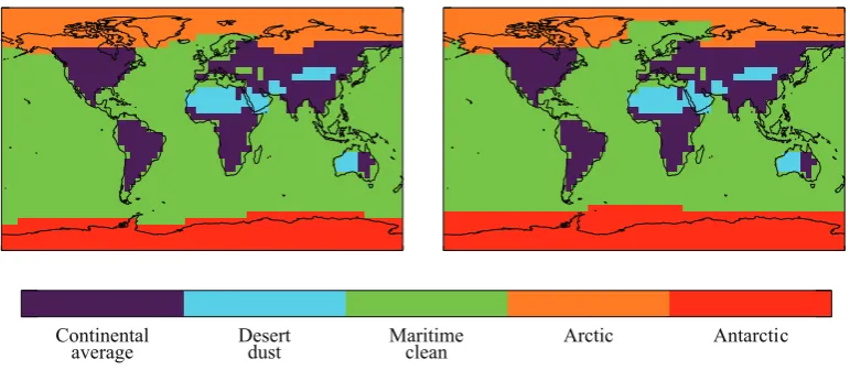
The configuration of the ORAC processor used in the GRAPE project uses channels 2–4 of the ATSR-2 instrument (centred on wavelengths of 0.67, 0.87 and 1.6µm). The 0.55µm channel is not used, as over the oceans it is either disabled, or in a narrow-swath (where the swath width of the instrument is reduced from 512 to 256 km), due to down-link bandwidth limitations of the ERS-2 satellite. The retrieval assumes an aerosol type based on the geographic location of each pixel and time of year, as shown in Fig. 1, with the pos-sible types being maritime clean, continental average, desert dust, Arctic and Antarctic classes from the OPAC database.

The retrieval of parameters at 550 nm when the retrieval does not utilise a measurement at this wavelength may in-tially appear strange and it might be presumed that the τa andRSare actually being retrieved at 670 nm (or some other wavelength) and then extrapolated to 550 nm. However, this is not the case. The optimal estimation retrieval fits all pa-rameters with all available measurements, weighted by S,

constrained by the assumed aerosol properties. Thus, al-though the inclusion of the 550 nm channel would undoubt-edly better constrain the retrieval and lead to smaller uncer-tainties on the retrieved parameters, the retrieved state would remain consistent with that retrieved without it.

It should be noted that the assumed aerosol microphysi-cal properties are a key source of uncertainty in all aerosol remote sensing applications and that describing the global distribution of aerosol with a small number of descrete classes is not a realistic reflection of its true diversity. Further more, our knowledge of typical aerosol properties

(7)

G. E. Thomas et al.: Aerosol retrieval algorithm 685

Figures

Continental

average Desertdust Maritimeclean Arctic Antarctic

Fig. 1. The spatial distribution of aerosol types used in the GRAPE aerosol product. The left map shows

the distribution used for Southern Hemisphere summer (October–March), the Northern Hemisphere summer

(April–September) is given on the right.

(a)

0.01 0.10 1.00 10.00

Effective radius (µm) 0.0

0.5 1.0 1.5 2.0

Optical depth

0.00 0.67 1.33 2.00

Optical depth

(b)

0.01 0.10 1.00 10.00

Effective radius (µm) 0.0

0.5 1.0 1.5 2.0

Optical depth

0.01 0.10 1.00 10.00

Effective radius

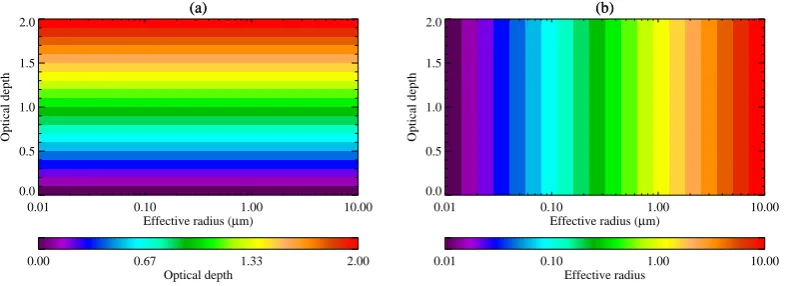
Fig. 2. The optical depth and effective radius fields used to produce simulated radiances for the ORAC retrieval.

The ranges have been chosen to span the full range of optical depths and effective radii covered by the ORAC

look-up tables. Ideally, the retrieval should reproduce these plots when applied to the simulated radiances.

31

Fig. 1. The spatial distribution of aerosol types used in the GRAPE aerosol product. The left map shows the distribution used for Southern Hemisphere summer (October–March), the Northern Hemisphere summer (April–September) is given on the right.

in different regions is improving continuously, particularly thanks to Alumcantar retrievals from Aerosol Robotic Net-work (AERONET) measurements (Dubovik et al., 2002), and some of the classes within the OPAC database (partic-ularly those which contain absorbing components) are now known to be inaccurate. However, the small number of chan-nels used in the GRAPE retrieval means that there is not enough information available to the retrieval to enable differ-ent aerosol types to be distinguished. The magnitude of the errors introduced by this simplistic assumption of the aerosol optical properties is investigated in Sect. 3.3.

Absolute measurement uncertainties are set at fixed val-ues of 0.005, 0.009, and 0.018 for channels 2, 3 and 4. For average cloud-free radiances these errors correspond to er-rors of approximately 2, 3 and 10% for each channel, respec-tively. These values were determined for cloud retrievals but are in line with the expected noise on ATSR-2 measurements (Smith et al., 2002), except for channel 4 where it is an over-estimate. The larger uncertainty on channel 4 was originally set because it was not subjected to the same pre-launch cali-bration applied to the other channels. The use of fixed mea-surement errors simplifies the retrieval code somewhat, but subsequent applications of ORAC retrieval will implement a more rigerous scheme, based on the magnitude of the mea-sured TOA reflectance and its spatial variablity.

Additional forward model error to account for both the Lambertian surface reflectance approximation and the con-straint of a fixed spectral shape to the surface reflectance is also included in Sat 20% of the a priori surface reflectance

and correlations between the channels (i.e. off-diagonal ele-ments in S) of 0.4. Again, these values were optimized for

the cloud retrieval.

The aerosol optical depth and effective radius are retrieved in log10space, while the surface reflectance is retrieved on a linear scale. The a priori and first guess surface albedo are set to the value defined by the sea-surface reflectance model over the ocean or the MODIS white-sky albedo over the land, with a 1σerror of 0.01. The a priori and first guess values for optical depth are set to log₁₀(τ )= −1.0±1.0, corresponding toτ=0.1 with 1σ error bounds of 0.01≤τ≤1.0. The a priori and first guess effective radius is set to the value prescribed in literature for each aerosol type, with error bounds of±0.5 in log₁₀(re). Table 2 summaries the state varibles and their

associated a priori. 3.1 Retrieval sensitivity

The foremost limitation on the performance of a retrieval sys-tem is the information content of the measurements them-selves and how sensitive each retrieved parameter is to per-turbations in the state. This limitation can be investigated by performing the retrieval on simulated data, so that all sources of forward model and forward model parameter error can be removed from the problem. Figure 2 shows the aerosol state parameters (optical depth and effective radius) which have been used to produce simulated ATSR-2 radiances using the optical properties of the OPAC maritime clean aerosol class. The retrieval has been run on these data, assuming the cor-rect aerosol class and with the a priori surface reflectance set to the correct value of 0.02. The a priori effective ra-dius for the maritime clean class is 0.832µm, giving 1σ er-ror bounds of 0.26<re<2.63µm. The results of applying

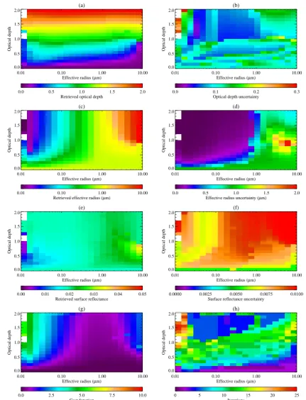
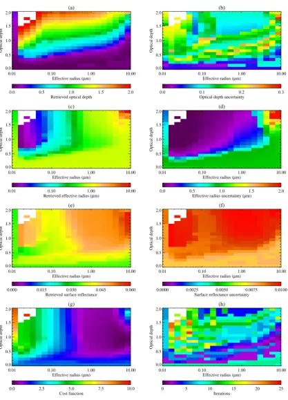
the retrieval to these data are given in Fig. 3, along with er-ror estimates derived from the diagonal of the state covari-ance matrix, the value of the cost function at the solution and the number of iterations required for convergence. The first thing to notice is that some retrievals have failed to converge

(8)

686 G. E. Thomas et al.: Aerosol retrieval algorithm

Figures

Continental

average Desertdust Maritimeclean Arctic Antarctic

Fig. 1. The spatial distribution of aerosol types used in the GRAPE aerosol product. The left map shows

the distribution used for Southern Hemisphere summer (October–March), the Northern Hemisphere summer (April–September) is given on the right.

(a) (a)

0.01 0.10 1.00 10.00 Effective radius (µm)

0.0 0.5 1.0 1.5 2.0

Optical depth

0.00 0.67 1.33 2.00 Optical depth

(b) (b)

0.0 0.5 1.0 1.5 2.0

Optical depth

0.01 0.10 1.00 10.00 Effective radius

Fig. 2. The optical depth and effective radius fields used to produce simulated radiances for the ORAC retrieval.

The ranges have been chosen to span the full range of optical depths and effective radii covered by the ORAC look-up tables. Ideally, the retrieval should reproduce these plots when applied to the simulated radiances.

31

Fig. 2. The optical depth and effective radius fields used to produce simulated radiances for the ORAC retrieval. The ranges have been chosen to span the full range of optical depths and effective radii covered by the ORAC look-up tables. Ideally, the retrieval should reproduce these plots when applied to the simulated radiances.

at the lowest effective radius (as indicated by white spaces in Fig. 3). This can be attributed to the optical depth being poorly constrained for the lowest size bin, as indicated by the large uncertainty estimates in its value (Fig. 3b). Poor performance of the retrieval in the lowest size bin is a re-curring theme in the results presented in this paper for this reason, and thus will not be discussed for each individual set of retrievals.

Figure 3g shows that the cost function at the solution has a value which is always less than 6. The smooth dependence on the state exhibited by the cost function is due to the a priori portion of the cost function ((x−xa)TSa−1(x−xa)):

i.e. the retrieval is fitting the measurements extremely well for all states, with the cost function being essentially deter-mined by the distance from the a priori. Statistically, one expects the cost function to follow aχ2distribution with a single degree of freedom3. This is not the case in this ex-ample, because the simulated measurements used in the re-trieval did not have noise added to them, while the rere-trieval was run using the error covariance matrix described earlier in this section. Thus the forward model can consistently fit the measurements more accurately than predicted by the mea-surement covariance matrix, S and the retrieved

uncertain-ties over estimate the error in the retrieval.

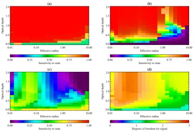
It is also very clear that the retrieval has failed to accurately estimate the true fields for states with low optical and large effective radius. To further explore why this is the case, we will examine the retrieval statistics further. Rodgers (2000) defines the averaging kernel for the maximum a posteriori solution as

A=SaKˆT

ˆ

KSaKˆT+S

−1

ˆ

K. (16)

3_{The cost function reported by ORAC is normalised by the} num-ber of measurements. If it were not, the degrees of freedom would equal the number of measurements (Rodgers, 2000).

Table 2. Retrieval state parameters and a priori assumptions. A

priori errors are given as 1σ.

State parameter a priori value a priori error

log₁₀(τa) −1.0 1.0

log₁₀(re) literature value 0.5 Rs MODIS over land, modelled over ocean 0.01

This matrix gives the sensitivity of the retrieved state to per-turbations in the true state,

Aij=

∂xˆj

∂xi

, (17)

wherexˆjis thejth element of the retrieved state andxiis the

ith element of the true state. The diagonal elements of this matrix can be thought of as an indication of the fraction of the retrieved state which can be said to be determined by the true value of that quantity (with the rest being determined by the choice of a priori and the value of the other elements of the state). For a perfect retrieval system A would be an iden-tity matrix, while a value of zero on the diagonal indicates that the corresponding state element is entirely determined by the a priori and values of the other state elements. The trace of the averaging kernel also gives the degrees of free-dom for signal for the given retrieval. This quantity gives the number of pieces of independent information retrieved. It is important to realise thatds is not a direct estimate of

the information content of the measurement, but rather in-dicates how much the measurement is able to improve our prior knowledge of the state. Figure 4 shows the diagonal elements of A, as well the overalldscorresponding to the

re-trieval shown in Fig. 3. The first thing to note is thatds.2.5,

indicating that the retrieved state is always somewhat influ-enced by the a priori. Looking at Fig. 4a–c, we can see that

(9)

(a)

0.0 0.5 1.0 1.5 2.0

Optical depth

0.0 0.5 1.0 1.5 2.0 Retrieved optical depth

(b)

0.0 0.5 1.0 1.5 2.0

Optical depth

0.0 0.1 0.2 0.3

Optical depth uncertainty

(c)

0.0 0.5 1.0 1.5 2.0

Optical depth

0.01 0.10 1.00 10.00 Retrieved effective radius (µm)

(d)

0.0 0.5 1.0 1.5 2.0

Optical depth

0.0 0.5 1.0 1.5 2.0 Effective radius uncertainty (µm)

(e)

0.0 0.5 1.0 1.5 2.0

Optical depth

0.00 0.01 0.02 0.03 0.04 0.05 Retrieved surface reflectance

(f)

0.0 0.5 1.0 1.5 2.0

Optical depth

0.0000 0.0025 0.0050 0.0075 0.0100 Surface reflectance uncertainty

(g)

0.0 0.5 1.0 1.5 2.0

Optical depth

0.0 2.5 5.0 7.5 10.0 Cost function

(h)

0.0 0.5 1.0 1.5 2.0

Optical depth

0 5 10 15 20 25

Iterations

Fig. 3. The retrieval results when the GRAPE algorithm is applied to the simulated data field with the correct

(OPAC maritime-clean class) aerosol optical properties. (a) and (b) show the retrieved optical depth and its

uncertainty respectively. Similarly, (c) and (d) show the retrieved effective radius and its uncertainty, while (e)

and (f) show the surface reflectance and its uncertainty. (g) shows the value of the cost function, Eq. 11, at the

solution and (h) shows the number of iterations required for convergence. White regions indicate where the

retrieval failed to converge.

32

Fig. 3. The retrieval results when the GRAPE algorithm is applied to the simulated data field with the correct (OPAC maritime-clean class) aerosol optical properties. (a) and (b) show the retrieved optical depth and its uncertainty, respectively. Similarly, (c) and (d) show the retrieved effective radius and its uncertainty, while (e) and (f) show the surface reflectance and its uncertainty. (g) shows the value of the cost function, Eq. (11), at the solution and (h) shows the number of iterations required for convergence. White regions indicate where the retrieval failed to converge.

(10)

688 G. E. Thomas et al.: Aerosol retrieval algorithm

(a) (a)

0.0 0.5 1.0 1.5 2.0

Optical depth

0.00 0.25 0.50 0.75 1.00 Sensitivity to state

(b) (b)

0.0 0.5 1.0 1.5 2.0

Optical depth

(c) (c)

0.0 0.5 1.0 1.5 2.0

Optical depth

(d) (d)

0.0 0.5 1.0 1.5 2.0

Optical depth

0 1 2 3

Degrees of freedom for signal

Fig. 4. The information content of the retrieval when applied to the simulated data field with the correct (OPAC

maritime-clean class) aerosol optical properties. (a)-(c) show the diagonal elements of the averaging kernel for optical depth, effective radius and surface reflectance, respectively. (d) shows degrees of freedom for signal (i.e. the trace of the averaging kernel) for each retrieval.

(a)

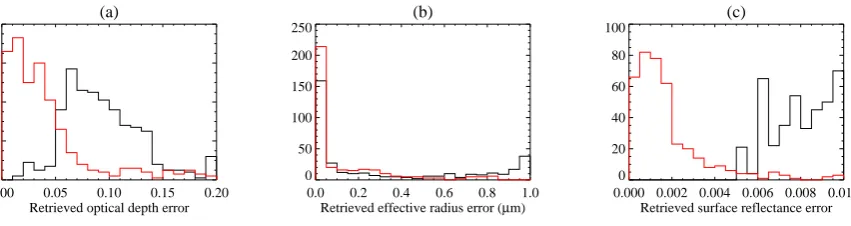
0.00 0.05 0.10 0.15 0.20 Retrieved optical depth error 0

20 40 60 80

(b)

0.0 0.2 0.4 0.6 0.8 1.0 Retrieved effective radius error (µm) 0

50 100 150 200 250

(c)

0.000 0.002 0.004 0.006 0.008 0.010 Retrieved surface reflectance error 0

20 40 60 80 100

Fig. 5. The black line shows distribution of retrieved uncertainties for each of the state parameters (i.e. standard

deviations taken from the state covariance matrix,Sˆ_{). The red line shows the distribution of the actual errors} (absolute difference between true and retrieved state). Note that 0.01 corresponds to the a priori error in the surface reflectance, which defines an upper limit on the retrieved uncertainty. The bin for the largest value includes all values greater than that bin, e.g. optical depths errors>₀.₁₉are included in the rightmost column of plot (a).

33

Fig. 4. The information content of the retrieval when applied to the simulated data field with the correct (OPAC maritime-clean class) aerosol optical properties. (a)–(c) show the diagonal elements of the averaging kernel for optical depth, effective radius and surface reflectance, respectively. (d) shows degrees of freedom for signal (i.e. the trace of the averaging kernel) for each retrieval.

in general optical depth is most sensitive to the measurement, as is effective radius at large optical depths, whereas the sur-face reflectance is mostly dominated by the a priori value.

It can also be seen that the regions of the domain where the retrieval has done least well (in particular, where optical depth is low and effective radius high) correspond to regions whereds is low and the effective radius shows poor

sensi-tivity to the true state. In such circumstances the effective radius is held at the a priori value and this results in an error in the retrieved optical depth, despite its good sensitivity to the true state.

Figure 5 shows the distribution of retrieved error estimates for each of the state elements, along with the distribution of the difference between the retrieved and true states. It can be seen that most retrievals provide optical depth to a preci-sion between 0.05 and 0.15, while the majority of effective radii have a precision of less than 0.1. It is clear that for most states, the retrieved optical depth is more accurate than indi-cated by the retrieved error estimate. As with the low values of the cost function shown in Fig. 3g, this can be explained by the fact that no measurement noise was added to the simu-lated radiances used in the retrieval. The retrieved error esti-mates give the 1σconfidence interval on the retrieved values, given the measurement and a priori uncertainties: since the simulated measurements actually contain no error, the accu-racy of the retrieval is substantially better than this estimate.

The effective radius errors show a similar pattern, although this is not apparent in Fig. 5b, due to the relatively coarse x-axis scale.

The surface reflectance error distribution shows somewhat different behaviour, since the retrieval used the correct value for the first guess and a priori. In addition, the surface re-flectance is retrieved on a linear scale, while the log₁₀of op-tical depth and effective radius are retrieved. Thus the maxi-mum of the retrieved surface reflectance error distribution is defined by the a priori error (while the retrieved error for op-tical depth and effective radius depends on the value of the retrieved state and hence has a relative, rather than an abso-lute, maximum). It is clear from Fig. 5c that the retrieval has somewhat narrowed the confidence interval on the value of surface reflectance for many states, but many more have not been improved at all.

Taken together, Figs. 3, 4 and 5 tell us several things about the retrieval:

– Overall, the retrieval is working well as there is an im-provement in our knowledge of almost all states (given by the narrowing of the uncertainties from their a pri-ori values) and the retrieved states almost always agree with the true value within uncertainty estimates. – The retrieval works best a high optical depths or

effec-tive radii between approximately 0.015 and 0.10.

(11)

G. E. Thomas et al.: Aerosol retrieval algorithm 689 (a)

(a)

0.01 0.10 1.00 10.00

Effective radius 0.0 0.5 1.0 1.5 2.0 Optical depth

(b) (b)

0.01 0.10 1.00 10.00

(c) (c)

0.01 0.10 1.00 10.00

(d) (d)

0.01 0.10 1.00 10.00

0 1 2 3

Degrees of freedom for signal

Fig. 4. The information content of the retrieval when applied to the simulated data field with the correct (OPAC

maritime-clean class) aerosol optical properties. (a)-(c) show the diagonal elements of the averaging kernel for

optical depth, effective radius and surface reflectance, respectively. (d) shows degrees of freedom for signal (i.e.

the trace of the averaging kernel) for each retrieval.

(a)

0.00 0.05 0.10 0.15 0.20 Retrieved optical depth error 0 20 40 60 80 (b)

0.0 0.2 0.4 0.6 0.8 1.0 Retrieved effective radius error (µm) 0 50 100 150 200 250 (c)

0.000 0.002 0.004 0.006 0.008 0.010 Retrieved surface reflectance error 0 20 40 60 80 100

Fig. 5. The black line shows distribution of retrieved uncertainties for each of the state parameters (i.e. standard

deviations taken from the state covariance matrix,

S

ˆ

_{). The red line shows the distribution of the actual errors}

(absolute difference between true and retrieved state). Note that 0.01 corresponds to the a priori error in the

surface reflectance, which defines an upper limit on the retrieved uncertainty. The bin for the largest value

includes all values greater than that bin, e.g. optical depths errors

>

₀

.

₁₉

_{are included in the rightmost column}

of plot (a).

33

Fig. 5. The black line shows distribution of retrieved uncertainties for each of the state parameters (i.e. standard deviations taken from the state covariance matrix,_{S). The red line shows the distribution of the actual errors (absolute difference between true and retrieved state).}ˆ

Note that 0.01 corresponds to the a priori error in the surface reflectance, which defines an upper limit on the retrieved uncertainty. The bin for the largest value includes all values greater than that bin, e.g. optical depths errors>0.19 are included in the rightmost column of plot (a).

– Where the retrieval is working well, optical depth and effective radius are both retrieved with a precision of

.0.1.

– The measurement is adding between 1 and approxi-mately 2.5 independent pieces of information to the system at this level of a priori constraint – i.e. the re-trieval is under-constrained, since we are attempting to retrieve more quantities than we have pieces of informa-tion from the measurement.

– Surface reflectance is poorly retrieved, with the a priori accounting for 50% or more of the retrieved value. Op-tical depth and effective radius show good sensitivity to the true state throughout most of the range.

– The strange feature in the effective radius fields above a true effective radius of ∼1µm (particularly evident in Figs. 3d and 4b) indicates a region of state space where effective radius is poorly constrained by the mea-surements. Corresponding patterns in the surface re-flectance fields indicate some degeneracy between these two variables. It is also notable that the optical depth retrieval remains quite stable throughout this region of state space.

The accuracy of the a priori surface reflectance also has a strong influence on the accuracy of the retrieved parameters. Although the GRAPE algorithm retrieves the magnitude of the surface reflectance, it is tightly constrained to the a pri-ori. This constraint is required because of the limited amount of information available in the measurements – if the surface reflectance is not tightly constrained, the retrieval is prone to converging on highly unrealistic states: i.e. the cost function has multiple minima. The effects of a 0.01 error (i.e. equal to the a priori error) and a 0.03 error in the magnitude of the a priori and first guess surface reflectance have been inves-tigated. A 0.01 error in surface reflectance produces results almost identical to those shown in Fig. 3, showing that the

retrieval is able to compensate for errors of this scale and fit the measurements as well and as quickly as when the correct a priori surface reflectance is used.

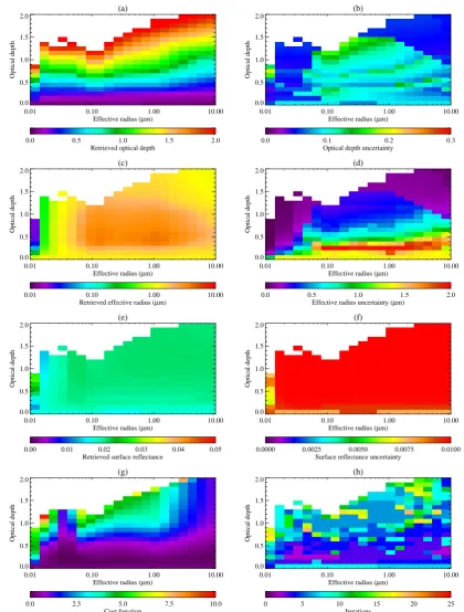
Fig. 6 shows the results of increasing the first guess and a priori surface reflectances to 0.05. In this case it is clear that the retrieval is unable to compensate for the larger dis-crepancy, particularly at either large, or the smallest effective radii, where the retrieved state is grossly different to the truth and the retrieved surface has not moved from the a priori value. Despite this the retrieved uncertainty estimates are similar to those in Fig. 3. Unsurprisingly, the retrieval deals with an error in the assumed surface reflectance better when the aerosol optical depth is high, as in this case the relative contribution of the surface to the overall signal is reduced. Figure 6g shows that for low effective radii, the cost func-tion is slightly higher, suggesting a poorer fit to the measure-ments; however for much of state space the cost is either sim-ilar or smaller than when the correct a priori is used. This, along with the low retrieval-error estimates, demonstrates the degeneracy in the retrieval system: the effect of the incorrect surface reflectance can be compensated for by changes in op-tical depth and effective radius.

These results indicate that the retrieval is able to compen-sate for errors in the a priori surface reflectance of the order of the a priori error, but not much larger than this. Unfor-tunately the retrieved state is still consistent with the mea-surements and a priori (as indicated by very similar retrieval costs) in both of these cases, meaning that it would not be possible to detect instances of poor a priori surface character-isation from the retrieval itself. However, it should be noted that cases of grossly inaccurate surface characterisation will be evident from the retrieval results, since it will not be pos-sible to correct for the surface reflectance by altering aerosol parameters. In such cases the retrieval will fail to converge, or will return an anomalously high cost.

(12)

690 G. E. Thomas et al.: Aerosol retrieval algorithm 3.2 Forward model errors

The term forward model error refers to inaccuracies that re-sult from incomplete or incorrect modelling of the relevant physical processes by the forward model. In the case of ORAC, these can be divided into four main categories:

1. Errors in modelling the scattering from the aerosol it-self; in particular, from the assumption of sphericity im-plicit in the use of Mie scattering.

2. Errors resulting in the discrete ordinates radiative trans-fer approach, including the assumption that the surface acts as a Lambertian reflector and the plane-parrallel ap-proximation.

3. Assumptions made in the formulation of the forward model expression (Eq. 10) used in the retrieval. 4. Interpolation errors due to the use of discrete

look-up tables for the transmission and reflectance terms in Eq. (10).

As mentioned in Sect. 2, the first of these sources of error is not addressed in this paper, although work is ongoing to investigate its effects and incorporate non-spherical scatter-ing into the ORAC system. The modellscatter-ing of atmospheric gas absorption, emission and Rayleigh scattering is another potential source of error, but the authors are confident that this is a minor contribution, particularly in the case of the ATSR instruments and SEVIRI, where the radiance error due to the assumptions made in the forward model is significantly smaller than the random error on the measurements. Simi-larly, the error introduced by the plane-parrallel approxima-tion will be minor, as the retrieval is not run when the view-ing geometry is such that this approximation is inaccurate. It should be noted that forward model error is unavoidable, es-pecially if the retrieval algorithm is to be reasonably compu-tationally efficient. As long as the sum of the forward model errors are kept well below the measurement noise level, how-ever, their effects will be minimal.

The error due to the DISORT radiative transfer will be dominated by the Lambertian surface reflectance approxima-tion, except at high zenith angles (>75◦) where the plane-parallel assumption of DISORT breaks down. This is a well known limitation of the DISORT method and is avoided by only running the retrieval on data which meets the plane par-allel criterion. In order to investigate the effect of the Lam-bertian surface approximation, DISORT was used to model TOA reflectances (following a similar procedure to the cal-culation of the look-up tables) for both a bi-directional sur-face reflectance and an equivalent Lambertian reflectance. The MODIS BRDF product was used to provide a variety of surface reflectances which span the typical range for land surfaces (the ocean surface reflectance has been neglected in this analysis, but it is generally far more isotropic than land surfaces, except for areas effected by strong sun-glint).

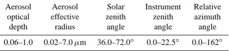
Table 3. The range of viewing angles and particle properties used in comparing DISORT and the GRAPE algorithm forward model. The range of viewing angles has been chosen to be typical for the ATSR instruments.

Aerosol Aerosol Solar Instrument Relative

optical effective zenith zenith azimuth

depth radius angle angle angle

0.06–1.0 0.02–7.0µm 36.0–72.0◦ 0.0–22.5◦ 0.0–162◦

The calculation was repeated for a wide range of view-ing geometries, aerosol loadview-ing and surfaces rangview-ing from desert to dense forest. Results show that the Lambertian approximation generally over-estimates the directional sur-face reflectance (which will dominate the TOA signal from the surface for typical background aerosol loadings) with the mean difference being 1.9% (median 1.4%) of the re-flectance, or, in absolute terms 0.002 (0.001). For a sur-face reflectance of∼0.25 (typical for a bright desert surface) the TOA reflectance using the Lambertian approximation is within 0.015 of the BRDF for all viewing geometries.

The latter two of the error terms listed at the beginning of this section can be quantified by comparing TOA reflectances computed directly from DISORT to those computed using the look-up tables and the forward model equation. Point 3 can be investigated by comparing the two qualities for view-ing geometries and aerosol properties which correspond to points in the look-up tables (so that no interpolation is re-quired). Point 4 can then be examined by doing the com-parison for values which lie half-way between the look-up table points (where interpolation errors can be expected to be maximum). This procedure has been followed for 4500 points across a wide range of viewing geometries and parti-cle states, as summarised in Table 3.

For values coincident with the look-up table points the for-ward model and DISORT agree to within±0.2% for 95% of viewing geometry and aerosol loading combinations, and al-ways agree to within±0.6%. There is, on average, a small positive bias apparent in the forward model expression, with the mean difference being 0.14% (median 0.14%). However, it is clear that for a Lambertian surface, Eq. (10) reproduces the DISORT modelled TOA radiances well.

Comparisons made for values where the effects of look-up table interpolation are maximised show that the interpolation error can far out-weigh that from the approximations made in Eq. 10. In some instances, it is possible for interpolation to introduce over 5% error into the modelled radiances, al-though for the vast majority of viewing angle/aerosol load-ing combinations the discrepancy is much lower than this. For this worst case ensemble of points the mean difference between the forward model and DISORT is −0.99% (me-dian−0.72%).

(13)

(a)

0.0 0.5 1.0 1.5 2.0

Optical depth

(b)

0.0 0.5 1.0 1.5 2.0

Optical depth

0.0 0.1 0.2 0.3

(c)

0.0 0.5 1.0 1.5 2.0

Optical depth

(d)

0.0 0.5 1.0 1.5 2.0

Optical depth

(e)

0.0 0.5 1.0 1.5 2.0

Optical depth

0.000 0.015 0.030 0.045 0.060 Retrieved surface reflectance

(f)

0.0 0.5 1.0 1.5 2.0

Optical depth

(g)

0.0 0.5 1.0 1.5 2.0

Optical depth

0.0 2.5 5.0 7.5 10.0 Cost function

(h)

0.0 0.5 1.0 1.5 2.0

Optical depth

0 5 10 15 20 25

Iterations

Fig. 6. Similar to Fig. 3. In this case the retrieval has been run using the correct aerosol optical properties, but

the first guess and a priori surface reflectances were set to 0.05, while the simulated radiances were generated

with a surface reflectance of 0.02.

34

Fig. 6. Similar to Fig. 3. In this case the retrieval has been run using the correct aerosol optical properties, but the first guess and a priori surface reflectances were set to 0.05, while the simulated radiances were generated with a surface reflectance of 0.02.

(14)

692 G. E. Thomas et al.: Aerosol retrieval algorithm Smith et al. (2002) quotes errors on ATSR-2

visible/near-infrared radiances as being between 1 and 5%, based on pre-launch calibration of the instrument and subsequent vicarious calibration of the visible channels using bright targets. Hence both the Lambertian surface approximation and look-up ta-ble interpolation can introduce errors which are larger than the measurement noise, with typical error values of the same order of magnitude.

3.3 Forward model parameter error

Forward model parameter error results from uncertainties in the parameters used in the computation of the forward model that are not included in the retrieval process. There are two main inputs into the modelled radiances which are most likely to significantly affect the output radiances:

1. The aerosol properties used in the calculation of the look-up tables (including the assumed size distribu-tion, refractive indices and vertical distribution of the aerosol).

2. The spectral dependence of the surface reflectance. In this section the effects on the retrieval of errors in a range of forward model parameters will be examined with a series of retrievals on simulated data, similar to that pre-sented in Sect. 3.1. The effects to be examined are:

1. The effect of using an inappropriate aerosol class. The GRAPE algorithm does not include any ability to re-trieve the composition of aerosol (aside from that im-plied by the change in composition that accompanies a change in effective radius) – it relies entirely on the accuracy of assumed optical properties, such as those provided by the OPAC database.

2. The effect of incorrect assumptions about the aerosol size distribution. Although the aerosol effective radius is retrieved, the form of the size distribution is fixed (to that defined in the OPAC database, for example). 3. The vertical distribution of aerosol used is an assumed,

fixed profile. One might assume that the TOA radiance in the visible is largely insensitive to the height distribu-tion of aerosol, but this should be quantified.

4. The effect of incorrect assumptions about the spectral dependence of the surface reflectance. Although the GRAPE algorithm is able to retrieve surface reflectance to a limited degree, it is only its magnitude which is per-mitted to vary. The spectral dependence is fixed at the a priori value.

Errors in any of these parameters will result in inaccuracies in the retrieved aerosol parameters. However, due to the non-linearity and complexity of the effects, and lack of knowl-edge about the accuracy of any one of them for a given re-trieval, it is not practical to attempt to characterise them with

standard Gaussian error statistics. Indeed it is not even mean-ingful to attempt to define “typical” values for such errors, since their effects are likely to be so variable. Thus, the ap-proach taken here is to test the retrieval in situations where the sources of error are completely known, in order to pro-vide indications of the magnitudes of each effect.

3.3.1 Incorrect aerosol properties

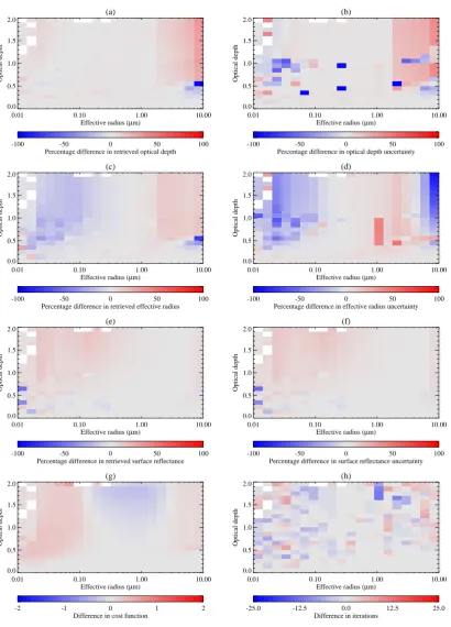
Figure 7 shows retrieval results when the GRAPE algo-rithm is applied to simulated radiances produced using the maritime-clean aerosol class from the states shown in Fig. 2, but using the OPAC desert dust aerosol class in the retrieval. It is encouraging to see that the optical depth field still shows a reasonable agreement with the input field. Overall how-ever, differences between the true and retrieved fields are much greater than when the correct aerosol properties are used in the the retrieval, particularly in effective radius. In this particular case, the use of the incorrect aerosol param-eters has resulted in differences in optical depth of between 10 and 30% for most states, while the effective radius shows typical differences of 100% or more. Despite this, the re-trieved uncertainties suggest a higher degree of confidence in the retrieved values than was the case with the correct aerosol class, with the uncertainties on optical depth in particular be-ing much smaller than in Fig. 3. Although this may seem a counter-intuitive result, it must be remembered that it simply indicates that the radiance shows a stronger dependence on aerosol optical depth for the desert aerosol class than for the maritime clean one. If the assumptions made in the retrieval are incorrect, the retrieved uncertainties cannot be assumed to be an accurate reflection of the acutal error in the result.

Overall the effect of assuming desert aerosol in place of maritime can be summarised as resulting in dramatic errors in retrieved effective radius, while the optical depth shows smaller perturbations. It is clear from Fig. 7 that the retrieved state alone does not provide enough information to determine whether the aerosol class used in the retrieval is appropri-ate – the retrieval has converged to reasonable values, with low costs, for the majority of the states tested. One might expect that if the aerosol optical properties assumed within the retrieval are incorrect, the forward model would not be able to provide a good fit to the measurements, resulting in the cost function having a higher value at the solution. How-ever, there is enough degeneracy in the system to allow incor-rect assumptions about the optical properties of the aerosol to lead to a retrieval which is consistent with the measurements and a priori.

If the assumed aerosol properties are very far from the truth however, the retrieval breaks down completely. For in-stance, applying the highly absorbing OPAC urban aerosol class to the simulated radiances generated from the maritime-clean class, results in the retrieval failing to converge for most high optical depths and those states which are retrieved have very large uncertainty estimates (on the order of 100%

(15)

(a)

0.0 0.5 1.0 1.5 2.0

Optical depth

(b)

0.0 0.5 1.0 1.5 2.0

Optical depth

0.0 0.1 0.2 0.3

(c)

0.0 0.5 1.0 1.5 2.0

Optical depth

(d)

0.0 0.5 1.0 1.5 2.0

Optical depth

(e)

0.0 0.5 1.0 1.5 2.0

Optical depth

0.00 0.01 0.02 0.03 0.04 0.05 Retrieved surface reflectance

(f)

0.0 0.5 1.0 1.5 2.0

Optical depth

(g)

0.0 0.5 1.0 1.5 2.0

Optical depth

0.0 2.5 5.0 7.5 10.0 Cost function

(h)

0.0 0.5 1.0 1.5 2.0

Optical depth

0 5 10 15 20 25

Iterations

Fig. 7. Similar to Fig. 3, except in this case the retrieval has been done assuming the OPAC desert aerosol class

rather than the maritime-clean one. Plots (a) and (b) show the retrieved optical depth and its uncertainty, (c) and

(d) show the effective radius and its uncertainty, while (e) and (f) show the surface reflectance and uncertainty.(g)

shows the cost function at the solution and (h) gives the number of iterations required for convergence.

35

Fig. 7. Similar to Fig. 3, except in this case the retrieval has been done assuming the OPAC desert aerosol class rather than the maritime-clean one. Plots (a) and (b) show the retrieved optical depth and its uncertainty, (c) and (d) show the effective radius and its uncertainty, while (e) and (f) show the surface reflectance and uncertainty. (g) shows the cost function at the solution and (h) gives the number of iterations required for convergence.