R E S E A R C H
Open Access
Analysis of pattern overlaps and exact
computation of P-values of pattern
occurrences numbers: case of Hidden Markov
Models
Mireille Régnier
1,7,8*, Evgenia Furletova
2,3*, Victor Yakovlev
2,5and Mikhail Roytberg
2,4,5,6Abstract
Background: Finding new functional fragments in biological sequences is a challenging problem. Methods addressing this problem commonly search for clusters of pattern occurrences that are statistically significant. A measure of statistical significance is theP-value of a number of pattern occurrences, i.e. the probability to find at least
Soccurrences of words from a patternHin a random text of lengthNgenerated according to a given probability model. All words of the pattern are supposed to be of same length.
Results: We present a novel algorithm SUFPREFthat computes an exactP-value for Hidden Markov models (HMM). The algorithm is based on recursive equations on text sets related to pattern occurrences; the equations can be used for any probability model. The algorithm inductively traverses a specific data structure, an overlap graph. The nodes of the graph are associated with the overlaps of words fromH. The edges are associated to the prefix and suffix relations between overlaps. An originality of our data structure is that patternHneed not be explicitly represented in nodes or leaves. The algorithm relies on the Cartesian product of the overlap graph and the graph of HMM states; this approach is analogous to the automaton approach from JBCB 4: 553-569. The gain in size of SUFPREFdata structure leads to significant improvements in space and time complexity compared to existent algorithms. The algorithm SufPref was implemented as a C++ program; the program can be used both as Web-server and a stand alone program for Linux and Windows. The program interface admits special formats to describe probability models of various types (HMM, Bernoulli, Markov); a pattern can be described with a list of words, a PSSM, a degenerate pattern or a word and a number of mismatches. It is available at http://server2.lpm.org.ru/bio/online/sf/. The program was applied to compare sensitivity and specificity of methods for TFBS prediction based onP-values computed for Bernoulli models, Markov models of orders one and two and HMMs. The experiments show that the methods have approximately the same qualities.
Keywords: P-value, Pattern occurrences, PSSM (PWM), Hidden Markov model
Background
The recognition of functionally significant fragments in biological sequences is a key issue in computational biology. Many functionally significant fragments are char-acterized by a set of specific words that is called a pat-tern and denotedHbelow. These patterns may represent
*Correspondence: [email protected]; [email protected] 1INRIA, d’Estienne d’Orves 1, 91120 Palaiseau, France
2Institute of Mathematical Problems of Biology, 142290, Institutskaya, 4, Pushchino, Russia
Full list of author information is available at the end of the article
different biological objects, such as transcription factor binding sites [1-3], polyadenylation signals [4], protein domains, etc. The functional fragments recognition prob-lem can be solved by finding sequences in which the words from a given pattern are overrepresented. Defining a meaningful significance criteria for this overrepresenta-tion is a delicate goal, that, in turn, requires a clarificaoverrepresenta-tion of the probability model. A current criteria is the so-calledP-value computed as the probability that a random sequence of lengthNcontains at leastSoccurrences of a pattern. There are many methods forP-value computation
designed for Bernoulli or Markov models. However, Hid-den Markov models (HMM) were considered in only a few papers [5,6] despite the models being widely used in bioinformatics. This is a motivation to develop methods forP-value calculation with respect to HMMs.
Existing methods forP-value calculation can be divided into several groups and reviews of the methods can be found in [7-10]. Studies on word probabilities started as early as the eighties with the seed paper [11] that introduced basic word combinatorics and derived induc-tive equations for a single word and a uniform Bernoulli model. Some works in the same vein, reviewed in [12] fol-lowed for several words, multi-occurrences and extended probability models. The time complexity is proportional to the text length N and the desired number of occur-rences S: computations are carried out by induction for n ranging over 1,. . .,N and, for a given n, by induc-tion on the number of occurrences. Although these “mathematics-driven” approaches allow for mathematical formula derivation, the actual computation suffers from a combinatorial explosion when |H| or Markov order increase.
Later on, a first group of methods [13-17] formal-ized systematically these inductions by the introduction of bivariate generating functions. Coefficients are theP -values to be computed. Expectations and variances for the number of occurrences of the different words in pattern
H can be expressed explicitly in terms of these gener-ating functions [14,15,18]. Moreover, coefficients may be computed from the analytical expression, when it is avail-able, or through a suitable manipulation of a functional equation, where the theoretical time complexity reduces toSlogN. Nevertheless, computing the generating func-tion, or the functional equafunc-tion, requires the computation of a system of linear equations or, equivalently, the deter-minant of a matrix of polynomials of sizeO(|H|). It takes O(|H|3) operations and it is the main drawback of this approach.
A second group of methods computes asymptotics. They rely on convergence results to the normal law proved by [19] or [20]. An approximatedP-value is derived, based on Gaussian approximations [21] or Poisson approxima-tions [22-25]. Nevertheless, this approximation is not suit-able for exceptional words, when the observed number of occurrences S significantly differs from the expected number. This was proved experimentally by [26] and theoretically [27]. Large deviation principles are used in [28,29] with a much better precision. Nevertheless, no computable formula are available for large sets.
A third group of methods revisits recursive P-value computation, with aO(S×N)time complexity. They avoid combinatorial explosion by a suitable use of appropriate data structures, tightly related to word overlap proper-ties. Therefore, loss in time dependency to N or S is
compensated by a gain on data structure size. A sig-nificant part of algorithms in this group are based on traversals of a specific graph. The graph may not be defined explicitly [30]. It can be based on the graph cor-responding to the finite automaton recognizing the given pattern, see algorithms AHOPRO[31], SPATT[25,32] and REGEXPCOUNT [17]. MOTIFRANK [33] that is designed for first order Markov models makes use of suffix sets. In [25,32,34], a Markov chain embedding technique was suggested. Counting occurrences of regular patterns in random strings produced by Markov chains reduces to problems regarding the behavior of a first-order homo-geneous Markov chain in the state space of a suitable deterministic finite automaton (DFA) [35,36]. In a recent paper [6], a probabilistic arithmetic automaton for com-putingP-values for a HMM was proposed. In this paper two algorithms were suggested. The first one has a time complexity O(|Q|2 × N × S × || × |V|) and a space complexity O(|Q| ×S × ||), where|Q| is the number of states of the HMM, || is the number of states of the automaton recognizing the given pattern, |V| is the alphabet size. The second algorithm has a time complexity O(|Q|3× log(N) × S2 × ||3) and a space complexity O(|Q|2×S× ||2). This algorithm uses the “divide and conquer” technique. The drawback is the lack of con-trol on the number of states || when |H| increases. Finally, despite these great efforts, existing methods per-form badly for rather big patterns. Besides this, most of the proposed algorithms are not implemented or imple-mented only for Bernoulli models or Markov models of small orders.
The present paper provides an algorithm supporting the HMM probability model. It assumes that all words have the same length m and that a HMM with |Q| states is given. It is a generalization of algorithm SUFPREFdesigned in [37] for Bernoulli models and Markov models of order K. It relies on recurrent equations based on an overlap graph, whose vertices are associated with the overlaps of words from H, and edges correspond to the prefix and suffix relations between overlaps. The time complexity is O(|Q|2×N×S×(|OV(H)|+|H|))and the space complexity is O(|Q|2×(|OV(H)|+|H|)+|Q|×S×m×|OV(H)|+m×|H|), where |OV(H)| is the number of overlaps between the words from the patternH. In the case of a Markov model of orderK, whereK≤m, bounds for time and space above can be reduced toO(N×S×(K×|V|K+1+|OV(H)|+|H|)) and to O(S×K× |V|K+1+S×m× |OV(H)| +m× |H|), respectively. Algorithm SUFPREF is implemented as a Web-server, see http://server2.lpm.org.ru/bio/online/sf/, and a stand-alone program for Windows and Linux. The program is available by request from the authors.
the Hidden Markov models definition. Main text sets are defined and equations for their probabilities are derived. The next section describes the algorithm SUFPREFthat computes these equations using the overlap graph as a main data structure. Then, the space and time complex-ities are analyzed and our algorithm is compared with other methods [3,24,31,38,39]. Finally, usage ofP-values for TFBS prediction is discussed.
Overlap words
Our approach strongly relies on overlaps of words from a given pattern. In this section we provide necessary definitions for these overlaps, following the notations of [37]. The main deference is in definition of over-lap graph, see definition 3. By definition from [37], overlap graph has additional nodes (leaves) that corre-spond to the words from the pattern H. In the present paper overlap graph has deep edges instead of the nodes. This modification is not affect on upper bounds of time and space complexity. But in practice it gives significant improvements.
Definition 1.Given a patternHover an alphabetV, a word w is an overlap(an overlap word)forHif there exist wordsHandFinHsuch that w is a proper suffix ofHand w is a proper prefix ofF. The set of overlaps of the pattern
His denoted OV(H).
Example 1.LetHbe the set
H= {ACAGCTA, ACATATA, CTTTCGC, TACCACA}.
The overlap set is
OV(H)= {, A, ACA, C, TA}.
Notation.Below we will use the following notations: 1)w, for an overlap fromOV(H); 2) H, for a word from the patternH; 3)v, for a word fromOV(H)∪H.
Notation.For an overlapwinOV(H), one denotes
H(w)= {H∈H|H ends withw} ,
with the conventionH()=H.
Notation.x x (x ⊂ x) means thatx is a suffix (proper suffix) ofx;x x(x≺x) means thatxis a pre-fix (proper prepre-fix) ofx. The elements ofOV(H)that are proper prefixes (respectively suffixes) of a given word are totally ordered. The empty string is the minimal element. The maximal elements are crucial for our algorithms and data structures.
Definition 2.Given a word v in OV(H)∪H\ {}, one denotes
lpred(v) = max{x|x∈OV(H)and x≺v}; rpred(v) = max{x|x∈OV(H)and x⊂v}.
Two words H and F from the pattern H are called equivalent if they satisfy
lpred(H) = lpred(F), rpred(H) = rpred(F).
Notation.Given two words x and w in OV(H), let H∗(x,w) denote the equivalence class consisting of all words H∈Hsuch thatlpred(H)=xandrpred(H)=w.
One notes, for a word H in H∗(x,w),
lpred(H∗(x,w))=lpred(H)andrpred(H∗(x,w))= =rpred(H).
(1)
LetP(H)denote the set of all equivalence classes onH.
Example 2.Consider the patternHfrom the previous example.
1. For the overlap ACA∈OV(H),lpred(ACA)=A, because A is the maximal prefix of ACA that is overlap. Analogously,rpred(ACA)=A.
2. The words ACAGCTA and ACATATA from the pattern are equivalent because
lpred(ACAGCTA)=lpred(ACATATA)=ACA and
rpred(ACAGCTA)=rpred(ACATATA)=TA.
These words are in the classH∗(ACA, TA). The partitionP(H)consists of three classes:
H∗(ACA, TA)= {ACAGCTA, ACATATA},
H∗(C, C)= {CTTTCGC}and
H∗(TA, ACA)= {TACCACA}.
Order relations are commonly associated to oriented graphs.
Definition 3.The overlap graph of a given patternHis an oriented graph where the set of nodes is OV(H)and the set of edges, E(H), contains theleft,rightanddeepedges, that are defined as follows:
• Aleft edgelinks nodexto nodewiffx=lpred(w);
• Aright edgelinks nodexto nodewiffx=rpred(w);
• Adeep edgelinks nodexto nodewiff there exists a non-empty classH∗(x,w)inP(H).
It is denoted OvGraph.
Definition 4.An overlap w ∈ OV(H) is called a left deep node, respectively a right deep node, if there exists a wordH∈Hsuch that w=lpred(H), respectively w=rpred(H). The sets of all left and right deep nodes are denoted by DLOV(H)and DROV(H).
Notation.For a right deep noder ∈ DROV(H), one denotes
H(r)= {H∈H|r=rpred(H)}.
Below we will userfor notation of a right deep node.
Definition 5.Let v be in(OV(H)∪H)\.
The set of non-empty prefixes of v (including v) that belong to OV(H)is denoted by OverlapPrefix(v). For any prefix x in OverlapPrefix(v), let Back(x,v)denote the suffix of v that satisfies the equation
v=x·Back(x,v).
Let Back(v)denote Back(lpred(v),v). Also forH∗(w,r)∈P(H)we denote
Back(H∗(w,r))= H∈H∗(w,r)
Back(H).
Remark.One can ascribe to each deep edge(w,r)the class H∗(w,r)and to each left edge(lpred(w),w)a word labelBack(w).
Example 3.The overlap graph for the pattern
H = {ACAGCTA, ACATATA, CTTTCGC, TACCACA}
is shown in Figure 1. The nodes of the graph correspond to the overlaps from the setOV(H)= {, A, ACA, C, TA}. The index numbers of nodes are the index numbers of overlaps in the prefix order. The graph has four left edges (shown by straight lines), five right edges (shown by dashed lines) and three deep edges (shown by double lines).
Text sets
The computation ofP-values will be done by induction on the text lengthn(n=1,. . .,N), and, for each givenn, by induction on the number of occurrencess(s=1,. . .,S).
It relies on formulas introduced in [37], that in turn was based on the ideas from [12,13]. In [37] we give formulas forP-values computation for Bernoulli and Markov mod-els. In the present paper we introduce equations on texts sets that underlie these formulas. Using these equations one can derive formulas forP-value computation for dif-ferent probabilities models. Also these equations take into account improvements in the overlap graph structure, see section “Overlap words”.
Figure 1Overlap graph for patternH= {ACAGCTA, ACATATA, CTTTCGC, TACCACA}.Nodes are the elements ofOV(H). The node with the index number “1” corresponds to, it is the root. The left edges are shown by continuous straight lines, right edges are shown by dashed lines and deep edges are shown by double lines. Each left edge(lpred(w),w), wherew∈OV(H), is labeled withBack(w). For example, edge(2, 3)corresponding to the pair of overlaps(A, ACA)is labeled withBack(ACA)=CA. A deep edge(w,r)corresponds to equivalence classH∗(w,r). The right edges(w,rpred(w))are not labeled.
Definition 6. LetHbe a pattern.
B(n,s)={t∈Vn|t contains at least s occurrences of the patternH}.
By convention, B(n, 0)=Vn.
Definition 7.Given a right deep node r ∈ DROV(H), one defines, for s=1,. . .,S,S+1
E(n,s,r)={t∈Vn|t contains at least s occurrences ofH& &t ends withH∈H(r)}
(2)
These sets are called E-sets.
Definition 8. Let w∈OV(H), one defines, for s=1,. . .,S
R(n,s,w)={t∈Vn|t contains exactly s occurrences ofH& &t ends withH∈H(w)}
(3)
These sets are called R-sets.
Remark.We remark that
Note, ift ∈ E(n,s,r) thent ends with a word H from
H(r), wherer = rpred(H). In contrast, ift ∈ R(n,s,w) then t ends with a word H from H(w), i.e. w is a suffix of H.
Example 4.Consider the patternH = {ACAGCTA,
ACATATA, CTTTCGC, TACCACA}from the example 1.
And consider the textt1=CTTTCGCCGAATCACAGCTA.
The texts is of length 20, contains exactly 2 occur-rences ofH(the occurrences are given in bold) and ends
with ACAGCTA. Obviously,rpred(ACAGCTA) = TA.
Thust1is inB(20, 1),B(20, 2),E(20, 1, TA),E(20, 2, TA), R(20, 2, TA),R(20, 2, A)andR(20, 2,).
Example 5.Consider the pattern H from the previ-ous examples and the set E(20, 2, TA). A text t from E(20, 2, TA)is of length 20, has at least 2 occurrences ofH and ends with a word H fromHsuch thatrpred(H)=TA. Obviously, H is ACAGCTA or ACATATA. The words ACAGCTA and ACATATA are from the same class H∗(ACA,TA). For example, textst1 = CTTTCGCCGA
ATCACAGCTA,t2 = CTTTCGCGGTACCACATATA,
t3 = TACCACATATACCACAGCTA, t4 = ACGTTT CCATACCACAGCTA,t5=ACTAAGACAGCTACATATA are inE(20, 2, TA). The occurrences ofHare given in bold or italic.
Definition 9.Given a right deep node r ∈ DROV(H), one defines, for s=1,. . .,S
RE(n,s,r)= {t∈R(n,s,r)|t ends withH∈H(r)}. (4)
Remark that
RE(n,s,r)=E(n,s,r)\E(n,s+1,r). (5)
Example 6.Consider the pattern
H1=H∪ATAGTCG= {ACAGCTA, ACATATA,
ATAGTCG, CTTTCGC, TACCACA},
where H is the pattern from the previous examples.
Obviously, OV(H1) = {, A, ACA, ATA, C, TA}.
Con-sider the textst1=CTTTCGCCGAATCACAGCTAand
t5 = ACTAAGACAGCTACATATA. The textst1andt5
belong toR(20, 2, TA)because the texts: 1) have length 20; 2) contain exactly two occurrences ofH1and 3) end with the words fromH1(TA), here TA is the suffix of the words. Also the textt1 is inRE(20, 2, TA) because it ends with
ACAGCTA, andrpred(ACAGCTA) = TA. In contrast,
t5is not inRE(20, 2, TA)because it ends with ACATATA, andrpred(ACATATA)=ATA.
The following proposition gives the inductive relations allowing effective computation of probabilities ofR-sets.
Proposition 1.Let w∈OV(H). If w is a deep right node, i.e. w=rpred(H)for a wordH∈H, then
R(n,s,w)=RE(n,s,w)∪ ⎛
⎝
x∈OV(H):w=rpred(x)
R(n,s,x) ⎞ ⎠,
(6)
otherwise,
R(n,s,w)=
x∈OV(H):w=rpred(x)
R(n,s,x). (7)
The proof follows from the definition ofR-sets.
Example 7.Lets illustrate the proposition 1 with the data from the example 6. As we have seen before, t1,t5 ∈ R(20, 2, TA). Further, t1 ∈ RE(20, 2, TA), and t5 ∈ R(20, 2, ATA). Here, TA = rpred(ATA). Also note, R(20, 2, ATA)=RE(20, 2, ATA).
Remark.For given n and s, we have to compute the probabilities of sets R(n,s,w) for all w ∈ OV(H). The equations (6) and (7) allow us to do this by recur-sive traversal of OV(H) from the leaves (deep nodes) of OvGraph to the root according to the right edges. The calculation starts from probabilities ofRE-sets found according to the equation (5).
Below we introduceD-sets and give the equations forD -sets,R-sets andE-sets leading to recursive equations for E-sets probabilities. TheD-sets defined below consist of texts of lengthncontaining at leastsoccurrences of the patternH, ending with a given non-empty overlap word wthat has a common part with thes-th occurrence of the patternH.
Definition 10.Let w∈OV(H), w=, k≥1. D(k,s,w) = {t∈B(k,s)|w is a suffix of t&
&s -th occurrence of the patternHintersects
the suffix w}. (8)
By definition, D(k,s,)= ∅.
Notation.Below we will use the following notations: 1)len(x), for the length of a wordx; 2)|M|, for the number of words in a set of wordsM.
Notation.For a prefixw ∈ OV(H)and any integern, one denotes
k(n,w)=n−m+len(w),
Example 8. Letn=20 ands=2. Consider the pattern
H = {ACAGCTA, ACATATA, CTTTCGC, TACCACA}
and the texts t4 = ACGTTTCCATACCACAGCTA,
t5 = ACTAAGACAGCTACATATAfrom the example 5.
In the both cases, the first occurrence ofHintersects the ending occurrence ofH. The texts end with words from the class H∗(ACA,TA)= {ACAGCTA, ACATATA}.
Consider the overlapw=ACA. Thenk(n,w)=16.
Con-sider the prefixes t4[1, 16]= ACGTTTCCATACCACA
and t5[1, 16]= ACTAAGACAGCTACA of the texts.
For these prefixes we have: (1) their length is 16; (2) the prefixes end with ACA; (3) the prefixes have at
least s − 1 = 1 occurrence of H and (4) the first
occurrence of H intersects the suffix ACA. Thus the
prefixes t4[1, 16] andt5[1, 16] are inD(16, 1, ACA). Fur-ther,t4andt5are inD(16, 1, ACA)·Back(H∗(ACA,TA)), whereBack(H∗(ACA,TA)) = {GCTA,TATA}. Note, that t5[1, 14] also belongs toD(14, 1, A).
The next propositions describe the relation between D-sets andR-sets.
Proposition 2.Let w∈OV(H), w=. Then
D(k(n,w),s,w)=
=
x∈OverlapPrefix(w)
R(k(n,w)−len(Back(x,w)),s,x)·Back(x,w).
(9)
Proof:[see Additional file 1].
Informally speaking,xis the common part of thes-th occurrence of the patternHin the textt∈D(k(n,w),s,w) and the suffixwof the textt. Remark that according to the definition 5: (1) is not inOverlapPrefix(w), (2)wis in OverlapPrefix(w).
Proposition 3.Let w∈OV(H)\, n≥m,s≥1. Then
D(k(n,w),s,w)=D(k(n,lpred(w)),s,lpred(w))× ×Back(w)∪R(k(n,w),s,w) .
(10)
Proof:Follows from the proposition 2 [see Additional file 1].
Corollary 1.Iflpred(w)=thenD(n,s,w)=R(n,s,w).
One observes that, whenevern<m,B(n,s)= ∅, and for allw∈OV(H)andr∈DROV(H),R(n,s,w)=E(n,s,r)= ∅. Now we are ready to formulate the main theorem of the section. The theorem gives recursive equations forB-sets andE-sets. The main equations (13)–(15) are based on the following observation. The set E(n,s+1,r),s ≥ 1,
can be divided in two disjoint sets: F(n,s + 1,r) and C(n,s+1,r). The setF(n,s+1,r)consists of such words thats-th occurrence of the pattern Hdoes not intersect the ending occurrence ofH. AndC(n,s+1,r)consists of those textstfromE(n,s+1,r)thats-th occurrence ofH intintersects the ending occurrence ofH.
Theorem 1.Let n≥m, s≥1and r∈DROV(H), i.e. r is a right deep node.
1. SetsB(n,s)andE(n,s,r)meet the following equations:
B(n,s) = B(n−1,s)·V∪R(n,s,) (11) E(n, 1,r) = Vn−m·H(r) (12) F(n,s+1,r) = B(n−m,s)·H(r) (13) C(n,s+1,r) =
w:(w,r)is a deep edge
D(k(n,w),s,w)×
×Back(H∗(w,r)) (14) E(n,s+1,r) = F(n,s+1,r)∪C(n,s+1,r) (15)
Note, that(w,r)is a deep edge iffH∗(w,r)∈P(H), see definition 3.
2. Unions (11), (14) and (15) are disjoint, i.e.
B(n−1,s)·V∩R(n,s,)= ∅ ;
if(w,r)=(v,x)then
D(k(n,w),s,w)·Back(H∗(w,r))∩D(k(n,v),s,v)× ×Back(H∗(v,x))= ∅;
F(n,s+1,r)∩C(n,s+1,r)= ∅.
Example 9. The statements (13)–(15) can be illustrated with the data from the examples 5 and 8. Letn=20,s=1, r=TA. Then (15) can be rewritten as
E(20, 2, TA)=F(20, 2, TA)+C(20, 2, TA).
Consider the textst1,. . .,t5from the example 5.
In each of the texts t1,t2,t3 the ending occurrence of the pattern does not intersect the first occurrence. There-fore the texts are in F(20, 2, TA). Note, that the ending occurrence ACATATA of the pattern int2intersects the second occurrence but not the first. Consider the prefixes oft1,t2andt3of lengthn−m=20−7=13,t1[1, 13]=
CTTTCGCCGAATC, t2[1, 13]= CTTTCGCGGTACC
and t3[1, 13]= TACCACATATACC. The prefixes con-tain at least one occurrence of H, i.e. the prefixes are in B(13, 1). Thus t1,t2,t3 ∈ B(13, 1) · H(TA), that is in agreement with the statement (13) of the theorem. Obviously,
H(TA)=H(TA)=H∗(ACA, TA)=
In contrast, in each of the texts t4 and t5 the last occurrence of the pattern intersects the first occurrence. Therefore the texts t4,t5 ∈ C(20, 2, TA). According to the example 7, the texts t4,t5 are in D(16, 1, ACA) · Back(H∗(ACA,TA)), that illustrates the statement (14) of the theorem.
Note, there is only one overlapwsuch thatH∗(w, TA)= ∅, that isw=ACA. Thus
C(20, 2, TA)=D(16, 1, ACA)·Back(H∗(ACA,TA)).
Proof:
1. Consider statement (11). A texttis inB(n,s)if and only if either its prefix of lengthn−1contains at leastsoccurrences ofHor as-th occurrenceHfrom Hends at positionn. In the first case,tis in
B(n−m,s)·V. In the second case, texttbelongs to
R(n,s,). The two cases are mutually exclusive; thereforeB(n,s)is a disjoint union and (11) is proved. 2. The statement (12) directly follows from the
definition ofE(n, 1,r). 3. Consider the statement (13).
(a) First, we prove that
F(n,s+1,r)⊆B(n−m,s)·H(r). When a texttis inF(n,s+1,r), it ends with a word
H∈Hsuch thatr=rpred(H), i.e.H∈H(r). The last occurrenceHof the pattern does not intersect thes-th occurrence in the textt. Thus the prefix oftof lengthn−mcontains at leastsoccurrences ofH, i.e. it is in
B(n−m,s), wheremis the length of pattern words. Thereforetis inB(n−m,s)·H(r). (b) Obviously, ift∈B(n−m,s)·H(r)then
• thas the lengthn;
• tcontains at leasts+1occurrences of the patternH;
• s-th occurrence ofHlies on the prefix of
tof lengthn−m, i. e. it does not intersect the last occurrence;
• tends withH∈H(r).
Thereforet∈F(n,s+1,r).
4. Consider the statement (14). LetYdenote the right side of equation (14).
(a) Prove thatC(n,s+1,r)⊆Y. If a texttis in
C(n,s+1,r)then it ends with a word
H∈H(r). The last occurrenceHintersects thes-th occurrence of the pattern in the text
t. LetH1be thes-th occurrence ofHint, and xbe the overlap betweenH1andHint.
Obviously,x∈OverlapPrefix(w), where
w=lpred(H), see definition 5 of
OverlapPrefix(w). The prefix oftof length
k(n,x), wherek(n,x)=n−m+len(x), contains exactlysoccurrences ofHand ends withH1, whereH1∈H(x). By definition ofR
-sets, the prefix is inR(k(n,x),s,x). Therefore
t∈R(k(n,x),s,x)·Back(x, H). Observing that
Back(x, H)=Back(x,w)·Back(H)
we obtain
t∈R(k(n,x),s,x)·Back(x,w)·Back(H).
Note,k(n,x)=k(n,w)−len(Back(x,w)), wherelen(Back(x,w))=len(w)−len(x). According to the proposition 2,
R(k(n,w)−len(Back(x,w)),s,x)·Back(x,w)⊆ ⊆D(k(n,w),s,w).
Thus
t∈D(k(n,w),s,w)·Back(H).
Note, ifH∈H∗(w,r)then
Back(H)⊆Back(H∗(w,r)). Therefore,
D(k(n,w),s,w)·Back(H)⊆D(k(n,w),s,w)× ×Back(H∗(w,r)).
This yields thatt∈Y.
(b) Proof thatY ⊆C(n,s+1,r). Lett∈Y, i.e
t∈D(k(n,w),s,w)·Back(H∗(w,r)). By the definition ofD-sets,
• thas the lengthn;
• tcontains at leasts+1occurrences of the pattern;
• s-th occurrence intersects(s+1)-th occurrence ofH;
• tends withH∈H(r).
Thust∈C(n,s+1,r).
5. The statement (15) follows from the definitions ofF
andC-sets.
Notation.Given two integers n and s, and a class H∗(w,r), one introduces
C(n,s+1,w,r)=D(k(n,x),s,w)·Back(H∗(w,r)); (16)
Obviously,
C(n,s+1,r)=
w: (w,r)is a deep edge
C(n,s+1,w,r).
Remark.The unions in equations (11), (14), (15) and (17) are disjoint. Therefore the probability of the set in the left part of an equation is the sum of probabilities of sets in the right side.
Probability models
We suppose that the probability distribution is described by a Hidden Markov Model (HMM). In this section, we recall some basic notions about HMMs and intro-duce the needed notations. In fact, it is shown in [6] that our definition is equivalent to the classical definition of HMM [40].
Definition 11. A HMM G is a triple G = Q,q0,π, where Q is the set of states, q0∈Q is an initial state, andπ is a function: Q×V×Q→[0, 1]such thatπ(˜q,a,q)is the probability, being in state ˜q, to generate symbol a and tra-verse to state q. For any state ˜q in Q, the functionπmeets the condition:
a∈V
q∈Q
π(˜q,a,q)=1 . (18)
A HMMGis calleddeterministicif for any(˜q,a)inQ×V there is only one stateqsuch thatπ(˜q,a,q) > 0. In this case the functionπcan be described with two functions:
1. a transition functionφ:Q×V→Q; 2. a probability functionρ:Q×V→[0, 1].
Namely,φ(˜q,a)is equal to the unique stateqsuch that
π(˜q,a,q) >0 andρ(˜q,a)isπ(˜q,a,q).
A HMMG = Q,q0,πcan be represented as a graph whereQis the set of vertices. Each edge is assigned with a labela∈V and with a probabilityp∈(0; 1]. There exists an edge from ˜qtoqwith the labelaand probabilitypiff
π(˜q,a,q) > 0 andp= π(˜q,a,q). The graph is called the traversal graph of HMMG.
Definition 12. Let h be a path in the traversal graph of the HMM G. The label of h is the concatenation of the labels of edges that constitute the path h. The probability Prob(h)of a path h is the product of the probabilities of the edges that constitute the path h.
Definition 13.The probability Prob(t)of a word t with respect to the HMM G is the sum of probabilities of all paths that start in the initial state q0and have the label t. Let q and ˜q belong to Q and t be a word. By definition, the probability Prob(˜q,t,q)to move from the state ˜q to the state q with the emitted word t is the sum of probabilities of all paths starting in the state ˜q, ending in the state q and having the word label t.
To describe effective algorithms related to HMMs, we need the notion of reachability.
Definition 14. Given a state ˜q and a word t, we define
ReachState(t,˜q)= {q|Prob(˜q,t,q) >0}.
Given a state q and a string t, we define
StartState(t,q)= {˜q|Prob(˜q,t,q) >0}.
A state q is called t-reachable from a state ˜q if and only if Prob(˜q,t,q) >0.
Definition 15.For a given word t, AllState(t)is the set of states that are reachable from initial state q0by at least one text with suffix t. For a set of words M,
AllState(M)=
t∈M
AllState(t).
Remark.
AllState(t)=
t∈V∗.t
ReachState(t,q0). (19)
Definition 16.Let w be an overlap word. We denote by PriorState(w,q) the set of states ˜q ∈ AllState(lpred(w)) such that q is Back(w)-reachable from ˜q, i.e.
PriorState(w,q)=AllState(lpred(w))∩ ∩StartState(Back(w),q);
Analogously, for each deep edge(w,r)and its associated classH∗(w,r), one notes
PriorState(H∗(w,r),q)=AllState(w)∩
∩ ⎡
⎣
H∈H∗(w,r)
StartState(Back(H),q) ⎤ ⎦.
HMM and probabilistic automata
The definition of HMM is very close to the definition of probabilistic automaton PA, [41,42]. The main difference lies in the interpretation of the behavior of a model. For a HMM, one considers a label as a symbol emitted by the HMM; for automata, one imagines an automaton that processes a given word letter by letter. Another difference connected with the previous one is that PAs are typically used to describe word sets; thus, for a given PA, the sub-set of accepting states is defined. HMMs are mainly used to describe probability models and thus have no accepting states.
a graph that represents our automaton are labeled with words rather than with letters, and thus it can be named a generalized probabilistic automaton, analogously to the definition of generalized HMM [44].
An originality of SUFPREFis that words from pattern
H, or classes, that represent terminal states in classical automata need not be explicitly represented. Neverthe-less, each class is uniquely associated to one deep edge.
Probabilities equations for HMM
In the section above the main text sets and corresponding equations were described. One can apply the equations to compute probabilities of the text sets for arbitrary probability models. Here we give formulas to compute the probabilities for an HMM. The formulas are based on the following observations. First, all unions in the text equations are disjoint. Second, an item of a set union is a set with already known probability or con-catenation of such sets. In the latter case the probability Prob(q1,L1·L2,q2)can be computed by the formula
Prob(q1,L1·L2,q2)=
˜q∈Q
Prob(q1,L1,˜q)·Prob(˜q,L2,q2),
(20)
whereProb(q,L,q)is a probability that, being in the state q, the chain will go to the stateqemitting a wordtfrom the setL.
Letn,sbe integers,w ∈ OV(H),r ∈ DROV(H) and q∈Q. Then
1. From (11) follows
Prob(B(n,s),q)= ˜q∈Q
Prob(B(n−1,s),˜q)·π(˜q,q)+
+Prob(R(n,s,),q),
(21)
whereπ(˜q,q)=a∈Vπ(˜q,a,q); 2. From (12) follows
Prob(E(n, 1,r),q)= ˜q∈StartState(H(r),q)
Prob(Vn−m,˜q)×
×Prob(˜q,H(r),q);
(22)
3. From (13)–(15) and (17) follows
Prob(F(n,s+1,r),q)=
˜q∈StartState(H(r),q)
Prob(B(n−m,s),q¯)×
×Prob(˜q,H(r),q);
(23)
Prob(C(n,s+1,w,r),q)=
=
˜q∈PriorState(H∗(w,r),q)
Prob(D(k(n,x),s,w),q¯)× ×Prob(˜q,Back(H∗(w,r)),q); (24)
Prob(E(n,s+1,r),q)=Prob(F(n,s+1,r),q)+ +
⎛
⎝
w: (w,r)is a deep edge
Prob(C(n,s+ 1,w,r),q) ⎞ ⎠;
(25)
4. Letlpred(w)=. Then from (10) follows
Prob(D(k(n,w),s,w),q)= ˜q∈PriorCloseState(w,q)
Prob(D(k(n,lpred(w)),s,lpred(w)),˜q)· ×Prob(˜q,Back(w),q)
+Prob(R(k(n,w),s,w),q);
(26)
Iflpred(w)=then
Prob(D(n,s,w),q) = Prob(R(n,s,w),q);
5. From (5) follows
Prob(RE(n,s,r),q)=Prob(E(n,s,r),q)− −Prob(E(n,s+1,r),q);
(27)
6. Letwbe a right deep node. Then from (6) follows
Prob(R(n,s,w),q)=Prob(RE(n,s,w),q)+
+ ⎛
⎝
x∈OV(H):w=rpred(x)
Prob(R(n,s,x),q) ⎞ ⎠;
(28)
Otherwise, from (7) follows
Prob(R(n,s,w),q)=
x∈OV(H):w=rpred(x)
Prob(R(n,s,x),q).
(29)
Algorithms
General description
algo-rithm SUFPREF, see Algorithm 1, computes the probability by induction on a text lengthn, wherem≤ n ≤N, and, for a givenn, by induction on a number of occurrencess, where 1≤s≤S.
The computation within the main loop is based on equations (21)–(29), related to B-sets,C-sets,F-sets, E -sets,D-sets,RE-sets andR-sets.
The computation related to texts of length n will be referred to asn-th stage of the algorithm’s work. The main computation within then-th stage is performed by depth-first traversal ofOvGraphfollowing left and deep edges. During the depth-first traversal for each visited node w ∈OV(H), the algorithm computes the probabilities of RE-sets and auxiliary probabilities ofD,F andC-sets by induction on number of occurrencess=1,. . .,S. Within the traversal we store the probabilities ofD-sets related to the nodes on the path from the root ofOvGraphto a cur-rent nodew, i.e. the nodesxfromOverlapPrefix(w), in the temporary arraysTempDProb(x,q)of the sizeS; the size of the data related to a nodexon the path isO(|Q| ×S), see sub-section “Main loop” below. Then update of auxiliary information stored in nodes ofOvGraph, namely, proba-bilities ofR-sets, is performed by a bottom-up traversal of OvGraphusing right edges.
Computation on the inductive equations relies on a generic procedure, analogous to theforward algorithmfor HMM [40], see also [5].
Preprocessing and data structures
On the preprocessing stage we initialize the global data structures of the algorithm, i.e. the OvGraph, including auxiliary structures assigned to its nodes and some other structures that are described at the end of this subsection.
Overlap graph The graph OvGraph is built from the
Aho-Corasick trie TH for the set H [45]. The nodes
belonging to the OvGraph correspond to the overlaps
and therefore can be easily revealed using suffix links of the Aho-Corasick trie, see [37] and [Additional file 2], for details of the procedure. The nodes of OvGraphare assigned with additional data (constant data and data to be updated at each stagen=m+1,. . .,N). All these data are initialized at the preprocessing stage, see below.
Constant transition probabilities related to nodes of overlap graph During the computation, algorithm SUF -PREFuses some probabilities that are constant and can be precomputed and stored.
• For each nodewand all statesqinAllState(w)and ˜q inPriorState(w,q), we store the “left transition probability”Prob(˜q,Back(w),q), see definitions 15
and 16. The left transition probabilities are used for the computation ofD-sets probabilities, see (26);
• Given a right deep noder, the “word probabilities”
Prob(˜q,H(r),q)are memorized for statesqin
AllState(r)and ˜q inQ. They are used to compute probabilities of theF-sets, see (23);
• Given a right deep noder, we store, for each class
H∗(w,r), the “deep transition probabilities”
Prob(˜q,Back(H∗(w,r)),q)whereqranges over
AllState(H∗(w,r))and ˜q ranges over
PriorState(H∗(w,r),q). The probabilities are needed for the computation ofC-sets probabilities, see (24).
The sets of statesAllState(w)andPriorState(w,q), left and deep transition probabilities and word probabilities are computed in a depth-first traversal along the left edges ofOvGraph[see Additional file 2].
Updatable probabilities related to nodes of overlap graph At the beginning of then-th stage, for each pair w,q, wherew∈OV(H)andq ∈AllState(w)we store a
(m−len(w))×SmatrixRProbs(w,q), where
RProbs(w,q)[i] [s]=Prob(R(l,s,w),q);
l ∈[k(n,w),n−1] ;s= 1,. . .,S;i= l mod(m−len(w)). The probabilities were computed at the previous stages. And the values in the matrices are updated at the end of then-th stage.
At the preprocessing stage, we compute the probabili-ties forn = 1,. . .,m;s = 1,. . .,S andq ∈ AllState(w) according to the formulas:
Prob(R(m, 1,w),q)=Prob(H(w),q);
ifn<mor (n=mands>1),
Prob(R(n,s,w),q)=0.
The global data unrelated to overlap graph Besides the data related to nodes ofOvGraphwe store the following data.
• Transition probabilities. For each ˜q,q∈Qwe store the constant probability
TransProb(˜q,q)=
a∈V
π(˜q,a,q);
At the beginning ofn-th stage, the following values computed at the previous stages are stored
• For eachq∈Q, updatable probabilities
Prob(Vn−m−1,q). They are used for computation of
Prob(E(n, 1,r),q)by the formula (22);
preprocessing stage, we compute the probabilities for
n=1,. . .,m,s=1,. . .,Sandq∈Qaccording to the formulas:
Prob(B(m, 1),q) = Prob(H,q);
Prob(B(n,s),q) = 0, ifn<m
or(n=mands>1).
Main loop
The aim of then-th stage (main loop, see lines 2–13 of the algorithm SUFPREF, see Algorithm 1) is to compute for all s=1,. . .,Sthe values
• Prob(B(n−m,s),q),n>2m;
• Prob(R(n,s,w),q)for allw∈OV(H),
q∈AllState(w).
To compute the probabilities Prob(R(n,s,w),q) the algorithm for each pair w,q, where w ∈ OV(H), q∈ AllState(w), uses local arrayTempRProb(w,q)of size S. Initially, for eachs,TempRProb(w,q)[s]=0.
The valuenis not changed within the main loop. The body of the loop consists of three parts.
Within the part 2.1, for all s = 1,. . .,S the val-ues Prob(B(n−m,s),q) are computed according to the formula (21); the values Prob(B(n − m − 1,s),q) and Prob(R(n−m,s,),q)were computed and stored at the previous stages.
The aim of the part 2.2 (procedure COMPUT
-EREPROB, see Algorithm 2) is to compute the values Prob(RE(n,s,r),q)for allr ∈ DROV(H),q ∈ AllState(r) ands=1,. . .,S.
The computation is performed using the recursive depth-first traversal ofOvGraphalong the left edges; it is based on the formulas (22)–(27). Let a nodewis visited, it corresponds to the call of COMPUTEREPROB(n,w). Firstly, COMPUTEREPROB computes Prob(E(n, 1,w),q) by the formula (22) and puts the values toTermRProb(w,q)[1].
Then by induction ons= 1,. . .,Sthe procedure com-putes the following probabilities.
Within the part B, see lines 8–14, for all states q∈AllState(w), the procedure computesProb(D(k(n,w), s,w),q) by the formula (26). To make the computation by the formula (26) one needs the value Prob(D(k(n, lpred(w)),s,lpred(w)),˜q); the value is stored in the array TempDProb(w,q), see sub-section “General description”.
Now consider the part C of Algorithm 2, see lines 15– 26. Although the calculation of probabilities ofR-sets and RE-sets is based on the formulas (25) and (27) we avoid explicit usage ofE-sets in our calculations. From (25) and (27) we have (heres>1)
Prob(RE(n,s,r),q)=Prob(E(n,s,r),q)−Prob(E(n,s+1,r),q)=
=Prob(F(n,s,r),q)+
+
w:(w,r)is a deep edge
Prob(C(n,s,w,r),q)−
−Prob(F(n,s+1,r),q)−
−
w:(w,r)is a deep edge
Prob(C(n,s+1,w,r),q)=
=(Prob(F(n,s,r),q)−Prob(F(n,s+1,r),q))+
+
w:(w,r)is a deep edge
(Prob(C(n,s,w,r),q)−Prob(C(n,s+1,w,r),q)).
Fors=1 we have
Prob(RE(n, 1,r),q) = Prob(E(n, 1,r),q)−Prob(E(n, 2,r),q)=
= Prob(E(n, 1,r),q)−Prob(F(n, 2,r),q)
−
w:(w,r)is a deep edge
Prob(C(n, 2,w,r),q).
The valueProb(E(n, 1,r),q)was computed and stored in TempRProb(w,q)[1] at the part A of the procedure. During the computation we accumulate the needed prob-abilities in the arrays TempRProb(w,q), see section C of the algorithm 2, lines 15–26. Visiting a left deep
node w, for each r such that there is a deep edge
(w,r), and for each q ∈ AllState(r), we firstly calcu-late the valueProb(C(n,s+1,w,r),q)using (24). Then add to the current value ofTempRProb(w,q)[s] the value Prob(C(n,s,w,r),q)−Prob(C(n,s+1,w,r),q)(ifs>1) or substract the valueProb(C(n, 2,w,r),q)(ifs=1).
In section D of the Algorithm 2, see lines 27–36 we analogously take into account the probabilities ofF-sets.
At part 2.3 of the algorithm SUFPREF
(proce-dure COMPUTERPROB, see Algorithm 3), the values
Prob(R(n,s,w),q)are computed according to the formulas (28), (29).
The computation is done by a recursive bottom-up traversal ofOvGraphalong the right edges. Also the pro-cedure records the computedProb(R(n,s,w),q) probabil-ities to the corresponding cells of the matrixRProb(w,q) and initializes elements ofTempRProb(w,q)by zeros.
Remark.The above traversals are implemented with a recursive procedure initially called at the root (node corresponding to) of OvGraph, see lines 11, 12 of the algorithm SUFPREF(Algorithm 1).
Post-processing
At the post-processing step of the algorithm (see Algorithm 1, lines 14–19),P-valueProb(B(N,S))follows by summation overQstates:
Prob(B(N,S))=
q∈Q
Algorithm 1:SUFPREF
Input: an alphabet V, HMMG=<Q,q0,π >, the lengthNof a random text, desired numberSof occurrences of pattern words, patternH
Output:Prob(B(N,S))
// 1. Pre-processing
1 Parsing of input data, creating ofOvGraph, initialization of data structures corresponding to the nodes ofOvGraph, computing ofB-sets andR-sets probabilities forn=m.
// 2. Main Loop
2 foreachn=m+1,. . .,Ndo
// 2.1. Computation of Prob(B(n−m,s),q) and Prob(Vn−m,q) 3 ifn>2mthen
4 foreachq∈Qdo
5 foreachs=1,. . .,Sdo
6 ComputeProb(B(n−m,s),q)using (21);
7 end
8 ComputeProb(Vn−m,q);
9 end
10 end
// 2.2. Computation of Prob(RE(n,s,r),q) for all
// s=1,. . .,S; r∈DROV(H); q∈AllState(r)
// using depth-first traversal of OvGraph following left edges
11 COMPUTEREPROB(n,);// see Algorithm 2
// 2.3. Computation of Prob(R(n,s,w),q) for all
// s=1,. . .,S; w∈OV(H); q∈AllState(w)
// using bottom-up traversal of OvGraph following right edges
12 COMPUTERPROB(n,);// see Algorithm 3
13 end
// 3. Post-processing
14 foreachn=N−m+1,. . .,Ndo
15 foreachq∈Qdo
16 ComputeProb(B(n,S),q)by the formula (21);
17 end
18 end
19 ComputeProb(B(N,S))by summation of the valuesProb(B(N,S),q);
Discussion
Space complexity The data stored consist of input data, temporary data used at the preprocessing step, the main data structureOvGraphand the working data unrelated to the OvGraph. The detailed description of all of the data is given in the section “Preprocessing and data struc-tures”. The space complexity is mainly determined by the memory needed for the data related to theOvGraphand temporary data used at the preprocessing step. We first briefly consider the data unrelated to the overlap graph; then we considerOvGraphdata. The input data consist of the text lengthN, the number of occurrencesS, a repre-sentation of an HMM and a patternH. The data related to
the pattern representation are included in the data related toOvGraphnodes and will be considered below. Storage size for an HMM isO(|Q|2×|V|). Thus the input data size isO(|Q|2× |V|).
Algorithm 2:COMPUTEREPROB
Input:integern,n>m; nodewofOvGraph
Output: arraysTempRProb(w,q)[] with probabilitiesProb(RE(n,s,w)), ifwis not right deep node then elements of TempRProb(w,q)[] are zeros
// 1. Computations
// A. Computation of Prob(E(n, 1,w),q)
1 if w is right deep nodethen
2 foreachq∈AllState(w)do
3 ComputeProb(E(n, 1,w),q)using (22);
4 PutProb(E(n, 1,w),q)toTempRProb(w,q)[1];
5 end
6 end
7 foreachs=1,. . .,Sdo
// B. Computation of Prob(D(k(n,w),s,w),q)
8 ifw=then
9 foreachq∈AllState(w)do
10 ComputeProb(D(k(n,w),s,w),q)using (26);
11 end
12 else
13 Prob(D(k(n,w),s,w),q)=0;
14 end
// C. Computation of Prob(C(n,s+1,w,r),q) 15 ifw is left deep nodethen
16 foreachdeep edge(w,r)do
17 foreachq∈AllState(r)do
18 ComputeProb(C(n,s+1,w,r),q)using (24);
19 ifs=1then
20 TempRProb(r,q)[1] –=Prob(C(n, 2,w,r),q);
21 else
22 TempRProb(r,q)[s]+=Prob(C(n,s,w,r),q)−Prob(C(n,s+1,w,r),q);
23 end
24 end
25 end
26 end
// D. Computation of Prob(F(n,s+1,w),q)
27 if w is right deep nodethen
28 foreachq∈AllState(w)do
29 ComputeProb(F(n,s+1,w),q)using (23);
30 ifs=1then
31 TempRProb(w,q)[1] –=Prob(F(n, 2,w),q);
32 else
33 TempRProb(w,q)[s]+=Prob(F(n,s,w),q)−Prob(F(n,s+1,w),q);
34 end
35 end
36 end
37 end
// 2. Recursion. Depth-first traversal of OvGraph following left edges
38 foreachx such that w=lpred(x)do 39 COMPUTEREPROB(n,x);
Algorithm 3:COMPUTERPROB Input:integern,n>m;w∈OV(H) Output: probabilitiesProb(R(n,s,w)), the
probabilities are stored in the matrices RProb(w,q),q∈AllState(w)
1 pos=nmod(m−len(w));
// Recursion. Bottom-up traversal of OvGraph following right edges
2 foreachx such that w=rpred(x)do 3 COMPUTERPROB(n,x);
4 foreachq∈AllState(x)do 5 foreachs=1,. . .,Sdo
6 TempRProb(w,q)[s]+=TempRProb(x,q)[s];
7 TempProb(x,q)[s]=0;
8 end
9 end
10 end
11 foreachq∈AllState(w)do 12 foreachs=1,. . .,Sdo
13 RProb(w,q)[s] [pos]=TempRProb(w,q)[s];
14 ifw=then
15 TempRProb(w,q)[s]=0;
16 end
17 end
18 end
The temporary data structures used by sub-algorithms in the preprocessing stage are released after their run-ning. Thus, the total memory used during this stage is O(|Q|2×(|OV(H)| + |H|)+m× |H|).
The working data unrelated toOvGraph consist ofB -sets probabilitiesProb(B(n−m−1,s),q)and probabilities Prob(Vn−m−1,q),q∈Q. These data needO(|Q| ×S)and O(|Q|)memory, respectively. Within the main loop we use local arrays withD-sets probabilities (the number of these arrays is at mostm× |Q|, see remark below) and arrays TempRProb(w,q)(for all w ∈ OV(H),q ∈ AllState(w)).
These arrays are of sizeS. Therefore the necessary memory to store all of the arrays isO(|Q|×S×m+|Q|×S×|OV(H)|). As we will see, all this memory, except for the memory needed to store Aho-Corasick trie, does not increase the space complexity of the algorithm.
Remark.During processing of a node win main loop one stores arrays withD-set probabilities for all left prede-cessors ofw, i. e. for allx∈OverlapPrefix(x). The number of left predecessors is bounded by the number of all pre-fixes of w, that is len(w), wherelen(w) ≤ m. Thus the number of arrays with D-sets probabilities used by the algorithm during the performing of main loop is at most m× |Q|.
Consider now the data related to the OvGraph. The
OvGraphstructure is determined by the patternH. The number of nodes and the number of left and right edges isO(|OV(H)|), that is upper bounded bym× |H|. How-ever, usually |OV(H)| ≤ |H|, see Table 1. The number of deep edges is equal to the number of classes,|P(H)|, that is upper bounded by|H|. Then the storage size for OvGraph isO(|OV(H)| + |H|). The data assigned to a node ofOvGraphconsist of constant data and updatable data. The constant data consist of left transition probabili-ties assigned to the nodes of theOvGraph, deep transition probabilities assigned to the deep edges and word prob-abilities assigned to the right deep nodes. The updatable data are probabilities ofR-sets assigned to all nodes. More precisely, left transition probabilities Prob(˜q,Back(w),q)
are stored in the memory associated with a node w;
deep transition probabilities Prob(˜q,Back(H∗(w,r)),q) are stored in the memory associated with deep edge(w,r); word probabilitiesProb(˜q,H(r),q)are stored in the mem-ory associated with a right deep node r. As a whole, it gives
O(|Q|2× |OV(H)|)+O(|Q|2× |P(H)|)+ +O(|Q|2× |DROV(H)|)≤
≤O(|Q|2×(|OV(H)| + |H|)).
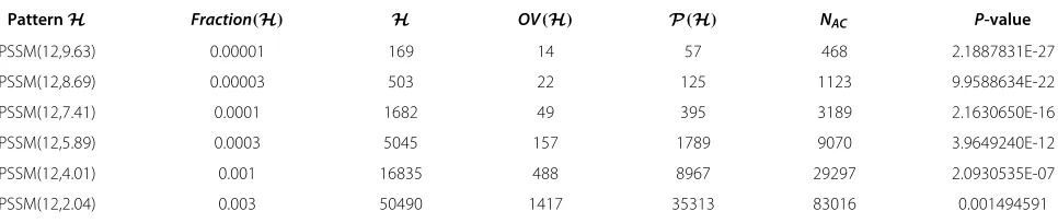
Table 1 PSSM-based patterns of length 12
PatternH Fraction(H) H OV(H) P(H) NAC P-value
PSSM(12,9.63) 0.00001 169 14 57 468 2.1887831E-27
PSSM(12,8.69) 0.00003 503 22 125 1123 9.9588634E-22
PSSM(12,7.41) 0.0001 1682 49 395 3189 2.1630650E-16
PSSM(12,5.89) 0.0003 5045 157 1789 9070 3.9649240E-12
PSSM(12,4.01) 0.001 16835 488 8967 29297 2.0930535E-07
PSSM(12,2.04) 0.003 50490 1417 35313 83016 0.001494591
To storeR-sets probabilities one needsO(S× |Q| ×m× |OV(H)|) memory. Thus the size of memory needed to store global data related toOvGraphis
O(|Q|2×(|OV(H)| + |H|)+ |Q| ×S×m× |OV(H)|). Finally, the overall space complexity of the algorithm is
O(|Q|2×(|OV(H)| + |H|)+ |Q| ×S×m× |OV(H)|+ +m× |H|).
Observe that the storage of classes in deep nodes saves aO(S× |Q| ×m× |P(H)|)memory forR-sets.
Remark.The parameter |OV(H)| belongs to the bounds of space and time complexities. It is upper bounded bym× |H|. Assume that a pattern consists of
random words of length m generated according to the
uniform Bernoulli model. It was shown that in such case |OV(H)| ≈ |H|, see [46] and supplementary materials, file “Comparison_with_AhoPro.xls”. But for a majority of patterns described by Position-Specific Scoring Matrices and cut-offs that were considered in the present paper, |OV(H)| ≤ 0.1 × |H|, see Table 1 in this paper and [Additional file 3].
Time complexity The algorithm SUFPREF (see
Algorithm 1) consists of three parts: preprocessing, main loop and post-processing. The time complexity of the pre-processing part is mainly determined by the construction of the Aho-Corasick trie and OvGraph, their traversals and the computation of intermediate probabilities. The complexity isO(|Q|2×m×(|OV(H)|+|H|). Some details are given in [Additional file 2]. The time complexity of the post-processing part (see lines 14–19) isO(m× |Q|2).
The time complexity of the algorithm SUFPREFis mainly determined by the main loop (see lines 2–13), i.e. by the total run-time of the computation of parts 2.1, 2.2 and 2.3 forn = m+1,. . .,N. Within the part 2.1 (lines 3–10), computing probabilities Prob(B(n − m,s),q) for all s=1,. . .,Sandq∈QrequiresO(S× |Q|2)operations.
Consider the part 2.2 (procedure COMPUTEREPROB, see Algorithm 2). The procedure performs computations by depth-first traversal ofOvGraphfor allw ∈ OV(H). For a givennandwthe computation consists of four parts: A, B, C and D. If wis right deep node then at the part A (lines 1–6) one computesProb(E(n, 1,w),q)for allq ∈ AllState(w); overall nodes this requiresO(|Q|2×|OV(H)|) operations.
The parts B, C and D run for S values of s. To exe-cute parts B, C and D (lines 8–14, 15–26 and 27–36
respectively) overall nodes of OvGraph one needs
O(S× |Q|2× |OV(H)|),O(S× |Q|2×(|OV(H)| + |H|)) andO(S× |Q|2× |OV(H)|)operations respectively.
As a whole,O(S× |Q|2×(|OV(H)| + |H|))operations are needed to execute COMPUTEREPROB.
Analogously, for computation of part 2.3 (see
pro-cedure COMPUTERPROB, see Algorithm 3) one needs
O(|Q|×S×|OV(H)|)operations. Therefore, the time com-plexity of the algorithm SUFPREFfor a general HMM is
O(N×S× |Q|2×(|OV(H)| + |H|)).
Time and space asymptotics In the previous sub-section we gave upper bounds of the space and time complexities of the algorithm SUFPREF. All bounds are given as big-O notations. For example, the time complexity bounds have formN×S×λ(G)×μ(H), hereNis the text length,Sis the number of occurrences,λ(G)is a factor depending on the HMMGandμ(H)is a factor depending on the patternH. The estimation of space complexity is analogous except of absence of factorN, see sub-section “Space complexity” for details.
In the case of a general HMMλ(G) = k× |Q|2, here |Q|is the number of states of the HMMG; the value ofk depends on features of the HMM.
We have performed computer experiments to get a better understanding of the asymptotic behavior of time and space complexity. LetNTransbe the number of states
where the HMM can transit in one step from a given state. This parameter describes the “density” of an HMM; the smaller NTrans, the smaller the complexities of the
algo-rithm. The factorλ(G)was studied as a function ofNTrans
and the number of statesNStatesin used HMMs. We have
performed 96=4×24 series of experiments, 100 exper-iments in each series. In all series we have used following input data:
• the pattern is defined by a PSSM for transcription factor FOXA2 from the database HOCOMOCO [47] and cut-off 5.89 that corresponds to roughly0.03%of all words of length 12;
• number of occurrences is 10;
• text length is 1000.
Thus, a series differs from the others only with the used HMMs. Each series is determined by the numberNState
of states in the HMMs, and the numberNTrans, see above.
The value NState ranges from 2 to 25, therefore 24
val-ues ofNStatewere considered. For each number of states
four values ofNTranswere used, namely, 1; 2; 0.25·NState
andNState. Given valuesNStateandNTrans, we have
cre-ated 100 HMMs by the following randomized procedure. For each state˜q, we firstly have randomly chosenNTrans
statesq ∈ Qsuch that there exists a transition from˜qto q. In our models if there exists transition from˜qtoqthen
![Figure 3 Average run-time of SUFPREF. The details of theexperiments are given in [Additional file 4]](https://thumb-us.123doks.com/thumbv2/123dok_us/341206.1526609/16.595.305.539.88.272/figure-average-time-sufpref-details-theexperiments-given-additional.webp)