10
ISSN 2307-4523 (Print & Online)
© Global Society of Scientific Research and Researchers
http://ijcjournal.org/
Satellite Image Classification Using Moment and SVD
Method
Mohammed S. Mahdi Al-Taei
a*,
Assad H. Thary Al-Ghrairi
ba,b
Dept. Computer Science, Al-Nahrain University, Iraq
a
Email: [email protected]
b
Email: [email protected]
Abstract
The motivation we address in this paper is to classify satellite image using the moment and singular value
decomposition (SVD) method; both proposed methods are consisted of two phases; the enrollment and
classification. The enrollment phase aims to extract the image classes to be stored in dataset as a training data.
Since the SVD method is supervised method, it cannot enroll the intended dataset, instead, the moment based
K-means was used to build the dataset. Thereby, the enrollment phase began with partitioning the image into
uniform sized blocks, and estimating the moment for each image block. The moment is the feature by which the
image blocks were grouped. Then, K-means is used to cluster the image blocks and determining the number of
cluster and centroid of each cluster. The image block corresponding to these centroids were stored in the dataset
to be used in the classification phase. The results of enrollment phase showed that the image contains five
distinct classes, they are; water, vegetation, residential without vegetation, residential with vegetation, and open
land. The classification phase consisted of multi stages; image composition, image transform, image
partitioning, feature extraction, and then image classification. The SVD classification method used the dataset to
estimate the classification feature SVD and compute the similarity measure for each block in the image, while
the moment classification method used the dataset to compute the mean of each column and compute the
similarity measure for each pixel in the image. The results assessment was carried out on the two classification
paths by comparing the results with a reference classified image achieved by Iraqi Geological Surveying
Corporation (GSC). The comparison process is done pixel by pixel for whole the considered image and
computing some evaluation measurements.
---
11
It was found that the classification method was high quality performed and the results showed acceptable
classification scores. In the SVD method, the score was about 70.64%, and it is possible to rise up to 81.833%
when assuming both classes: residential without vegetation and residential with vegetation is one class.
Whereas, the classification score was about 95.84% when using the moment method. This encourage results
indicates the ability of proposed methods to efficient classifying multibands satellite image.
Keywords: Satellite image classification; segmentation; blocbased classification; pixel-based classification; k-Means; SVD; Moment.
1.Introduction
Remote sensing uses satellite imagery technology to sense the landcover of Earth. At the early of 21st century,
satellite imagery became widely available with affordable [1]. Satellite image classification is the most
significant technique used in remote sensing for the computerized study and pattern recognition of satellite
information, which is based on diversity structures of the image that involving rigorous validation of the training
samples depending on the used classification algorithm [2]. It is an extreme part of remote sensing that depends
originally on the image resolution, which is the most important quality factor in images [3]. Image Classification
or segmentation is a partitioning of an image into sections or regions. These regions may be later associated with
ground cover type or land use, but the segmentation process simply gives generic labels (region 1, region 2, etc.)
to each region. The regions consist of groupings of multispectral or hyperspectral image pixels that have similar
data feature values. These data feature values may be the multispectral or hyperspectral data values and/or they
may be derived features such as band ratios or textural features [4]. The powerful of such algorithms is depends
on the way of extracting the information from huge number of data found in images. Then, according to this
information, pixels are grouping into meaningful classes that enable to interpret, mining, and studying various
types of regions that included in the image [3]. Many applications based on using Landsat imagery in a
quantitative fashion require classification of image pixels into a number of relevant categories or distinguishable
classes [5]. These applications use image classification as an important tool used to identify and detect most
relevant information in satellite images [6].
2.Related Work and Contribution
Many literatures devoted to image segmentation and classification. They differ in many aspects such as;
material images, used approach, or even the application limitations. The feasibility of using SVD for image
classification is investigated in the following:
2.1 Related Work
In [7], a neural network-based cloud classification were provided using the wavelet transforms (WT) and
singular value decomposition (SVD), in which the salient textural feature of the data was extracted. In [4], a
feed-forward neural network for satellite image segmentation, which provides a way to solve the problem of
parametric-dependence involved in statistical approaches using a robust, fault-tolerant, feed-forward neural
12
on clustering of the Kohonen’s self-organizing map (SOM), the implementation showed reasonable results. A
segmentation and classification of remote sensing images were established in [9], the classified image is given
to k-Means algorithm and back propagation algorithm of ANN to calculate the density count, the excremental
result found that k-means algorithm gives very high accuracy, but it is useful for single database at a time. Also,
an experimental survey for the SVD as an efficient transform in image processing applications performed in
[10], some contributions that were originated from SVD properties analysis in different image processing are
proposed. New method for satellite image classification was established in [11], there were multiple predefined
landcover classes, the results were accurate when describing different landcover regions in the test image. In
[12], an efficient image classification technique for satellite images was proposed, the work done with the aid of
KFCM and artificial neural network (NN), in spite of relatively long implementation time, the classification
results were valued. Furthermore, a cellular with fuzzy rules for classifying the satellite image was implemented
in [13], the quality of classified image was also analyzed, and the results indicate the ability of evolutionary
algorithms for classifying the satellite images. In [14], a combination of three classification methods was
proposed; these methods are the k-means, LVQ (linear vector quantization) and SVM (support vector machine),
such combination needed to modify some mathematical relationships that belong to the basic concepts of them,
the combination leads to long implementation time and high quality results. While [15] proposed a method for
area classification of Landsat7 satellite image using area clustering method, which is depends on pixel
aggregation after distributing some seeds in the test image, the assessment showed accurate classification result.
2.2 Contribution
Most of literatures are concerned with improving the classification methods for satellite images. The
contribution is described by improving the task of data enrollment instead of repeated interest in the process of
classification, which actually leads to improve the classification results. This requires using the SVD method
that usually needs to establish the dataset before starting the classification process. Such that, the proposed
method is based on the use of k-means based singular value decomposition (SVD), in which SVD is stand for
supervised method depending on predefined dataset stored in the dictionary that firstly established using the
k-means. The optimal run of training phase leads to create optimal dataset stored in the dictionary and then used to
determine intended classification results when the classification phase is running. Implies, the optimal choice of
the dataset indicates an optimal classification results.
3.Materials and Methods
Classification of satellite images can be achieved by unsupervised or supervised procedures, it is performed
when the image needs to be assigned into a predefined classes based on a number of observed attributes related
to that image. This refers to the task of extracting information from satellite image; the information is assigned
into classes according to specific features that distributed in the image [16]. The following sections introduce the
concepts of the used features: singular value decomposition (SVD) and moment besides the clustering based on
K-Means.
13
Singular Value Decomposition (SVD) is a mathematical tool widely in image classification; it is useful
factorizations method in linear algebra [17]. SVD technique is based on a theorem of linear algebra that
mentions; a rectangular m n matrix A having m rows and n columns in which m⩾n, is can be broken down into
the product of three matrices, as given in Equation (1) [18].
A= … (1)
Where U is a m n matrix of the orthonormal eigenvectors of AAT called the left singular vectors of A satisfy equation (2), VT is the transpose of a n n matrix containing the orthonormal eigenvectors of called the right singular vectors of A satisfy equation (3), and are the identity matrices of size n and p, respectively,
and S is a n n diagonal matrix with nonnegative diagonal entries of the singular values which are the square
roots of the eigenvalues of and called the singular values of A, which given in eq.(4) [19], as follows:
U= ... (2)
V= ... (3)
S=
Where σ1≥ σ2≥ · · · ≥ σp, p = min {m, n}, and U = V = . In such case, the SVD value
is the minimum value of diagonal terms, which can be used as a distinguished feature for any image segment.
3.2 K-Means Based Clustering
K-means is one of the effective unsupervised learning methods that solve the clustering problem. The
application of this algorithm on digital image requires being starts with some clusters of pixels in the feature
space, each of them defined by its center. The first step is randomly choosing a predefined number of clusters.
Second step is allocating each pixel to the nearest cluster. While, the third step is computing new centers with
new clusters. These three steps are repeated until convergence. Therefore, the k-means algorithm adopts the
following three steps till reaching the final state [9].
1. Determine the centroid coordinate.
2. Determine the distance of each object to the centroid.
3. Group the object based on minimum distance.
3.3 Moment Based Classification
The concept of moment is derived from Archimedes' discovery of the operating principle of the lever. In the
14
noted that the amount of force applied to the object (i.e., moment) is defined as
… (5)
Where F is the applied force, and r is the distance from the applied force to object and s is the order of the
moment. In image processing, the pixel value represents the force F, whereas r is the distance between the pixel
and the center of the moment. The moment gives an actual indication about the contents of an image or image
segment, such that it is used to distinguish different image segment from each other. Also, it is used to describe
details of small areas found in the image, which is a useful for image classification [20].
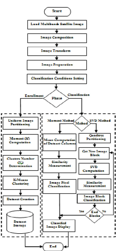
4.Proposed Classification Methods
The generic structure of the proposed method for satellite image classification using K-means based SVD is
shown in Figure (1). It is shown that the proposed method is designed to be consisted of two phases: enrollment
and classification. The enrollment phase goes to collect the training dataset (referred as A), which an offline
phase is responsible on collecting sample image classes to be stored in dataset matrix to be a comparable
models. Whereas the classification phase is an online phase responsible on verifying the contents of the test
image in comparison with the trained models found in the dataset, this phase depends on the dataset created by
the enrollment phase. Both phases are composed of the three preprocessing stages include: image composition,
image transform and preparing. Then, the enrollment includes sequenced stages of image partitioning, feature
extraction and then clustering to establish the dataset. On the other hand, the classification phase consist of
sequenced stages aims to extract the classification features from the employed image unit. In addition, there are
an intermediate stages included in the classification are used to achieve the intended purpose are shown in
Figure (1) and described in the following sections.
4.1 Image Composition
Satellite image is usually taken in multibands; this stage is aiming to compose the most informatic three bands
in one color image given in RGB color space. The dispersion coefficient (D) of the whole image f (i,j) that given
in equation (6) is used as a measure for quantifying whether a set of observed details are clustered or dispersed
compared to a standard case. This parameter indicates the amount of the information found in each band. The
three bands of greatest value of D are chosen to be combined with each other to make the composed image
FR,G,B(i, j) employed in the following stages.
... (6)
Where, and are the mean and variance of kth band of satellite image of W H resolution as given in equations (7 and 8). Such that, the green band FG, red band FR, and blue band FBare assumed to be the first three
bands that possess maximum dispersion coefficient Dk as given in equations (9-11):
15
… (8)
... (9)
... (10)
... (11)
4.2 Image Transform The three estimated bands FR, FG, and FB are converted into newly bands according to YIQ color transformation system. The Y represents the intensity band, whereas both I and Q represent the chrominance bands. Just the Y band is useful in the present work, which can be noted as FT and estimated according to the following relation: FT(i,j)=0.2989 FR(i,j)+0.5870 FG(i,j)+0.1140FB(i,j) ... (12)
4.3 Image Preparation This stage is regarded to increase the contrast of the given material image. Contrast stretching is used to enhance the appearance of image details, which can be achieved by adopting the linear fitting applied on the input image FT for achieving the output image FP as given in the following equation: FP=aFT+b … (13)
Where, a and b are the linear fitting coefficients given in the following equations, in which Min1 and Max1 are the minimum and maximum values of pixels found in transformed image, whereas Min2 and Max2 are the intended values of the minimum and maximum of output image pixels. … (14)
… (15)
4.4 Classification Conditions Setting
In this stage, the intended conditions of classification status are determined. This conditions are used in both
enrollment and classification phases. For the partitioning stage, the maximum block size (BMax) and minimum
block size (BMin) are set at the situation that gave best classification results. This depends on the number of try
making for achieving best results.
4.5 Enrollment Phase
16
classes depending on sequenced stages. It is intended to uniformly partition the prepared image (FP) into equal
blocks of size BMax. The reason of using BMax is to make the dataset containing greater number of information
related to each class, and make the moment is the feature that recognizes each part. K-Means algorithm is used
for grouping these features and then determining the best clusters (centroids) within the resulted features. The
image part belongs or closes to each centroid are stored in dataset array to be used in the classification phase.
This dataset can resized and scaled down to be half or quarter BMax as needed in the classification. The average
of the two successive elements gave new value in the half scaled down dataset, and another averaging leads to
get quarter scaled down for the dataset.
17
The Moment is a specific quantitative measure used to represent the information found in each image block. The
shape of a set of pixels is a distribution of mass, which can be described by first-ordered moment given in
equation (5), where the applied force (FP) represented the pixel of block and r is the distance from the applied
force to the center of block. In such case, the pixel value (FP) is regarded as the meant force, while the distance
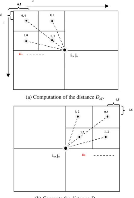
(Ds) is determined depends on the position of each pixel (In first, second, third, or fourth quarters) as shown in
Figure (2). The moment of each block can be determined as shown below:
1. Compute the Euclidean distance Ds between each pixel of a specific block and the center of that block
(the difference between the pixel and the center of block) as follows:
a. If the pixel FP(i, j) falls in the First quarter then the Ds1 is computed by using the following relation:
Ds1 = … (16)
b. If the pixel FP(i, j) falls in the Second quarter then the Ds2 is computed by using the following relation:
Ds2 = … (17)
c. If the pixel FP(i, j) falls in the Third quarter then the Ds3 is computed by using the following relation:
Ds3 = … (18)
d. If the pixel FP(i, j) falls in the Fourth quarter then the Ds4 is computed by using the following relation:
Ds4 = … (19)
Where , are represent the indices of the center block.
2. Compute the moment Mp (i, j) of each pixel in a specific block of image by using the following
relations:
Mp (i, j) = FP (i, j)x Ds … (20)
3. Compute the moment of a specific block (M) in image by using the following relation:
M = … (21)
Where Bh is the height of block and Bw is the width of block, M (i, j) represent the moment of pixel in a specific
block of image, and FP (i,j) represent the pixel value of a specific block at position (i,j), i, and j are indices of the
18
Figure 2: Schematic description for for computing the distance DS for cases (a and b), which are similar to cases (c and d).
The implementation of K-Means depends on two input parameters, they are; the number of clusters (or
classes) and the moment values of each block in the image. Actually, the number of classes (NC) in the prepared
image is determined in the following steps:
1. Determine the number of pixels in satellite image NT by using the following relation:
NT =W H … (22)
Where W represents the width of satellite image and H represents the height of satellite image.
2. Determine the standard deviation (𝛔𝛔) to prepare image that is by employing equation (8) to be modified
in the following form:
𝛔𝛔 = … (23)
1,0 1, 1
0, 1
DS1
(a) Computation of the distance Ds1.
io, jo
0, 0
i
j 0.5
0.5
(b) Compute the distance Ds2. 1, 2
0.5 0, 2
Ds2
0,3 0.5
1,2
19
Where is the mean of the prepared image that can be computed by the following relation:
… (24)
3. Calculate the number of pixels N in the image that fall within the range of 2𝛔𝛔 in the image distribution. 4. Compute the percent (P) of the pixels number (N) in 2𝛔𝛔 expansion and the number of pixels in whole
image (NT) by using the following relation:
… (25)
5. The number of classes (NC) is equal to the multiplication of the percent (P) by the maximum probable
number (PM) of classes may found in the satellite images, as follows:
NC= P PM … (26)
Dataset Formatting and Storing deals with output centroid of K-Means algorithm. The image block
corresponding or closest to centroid moment is stored in two dimensional dataset array (A), in which each block
is converted into one dimensional vector to be one column in A. Such that, the width of A is the number of
classes (Nc) while the height of A is equal to the number of pixels found in the block (i.e., BMax BMax).
4.6 Classification Phase
The classification phase is carried out after performing the training phase (enrollment). It can be achieved by
two paths: SVD method (block-based classification) or Moment method (pixel-based classification). The SVD
method path depends on the established dataset array A, where the prepared image is segmented into
non-uniform blocks and then each block is assigned to the dataset array A to compute the classification feature.
According to this feature, the block is labeled with available classes. Whereas, the moment method path depends
on the proximity of each pixel into the available classes in the dataset array A. The following subsections
explain more details about the two classification paths:
A. SVD Classification Phase
Since the SVD classification method needs to partition the image into predefine sized image block, where the
SVD classification phase used the quadtree to segment the prepared image into non uniform blocks restricted
between BMax and BMin. Then each square either leaved as it or subdivided into four quadrants when it satisfies
the partitioning conditions. Then, each block is assigned to the dataset array A to compute the classification
feature. According to this feature, the block is labeled with available classes. Since the SVD classification
method needs to partition the image into predefine sized image block, quadtree partitioning method is used for
segmenting the image into addressed image blocks. Therefore, the implementation of quadtree partitioning
method requires to set some parameters are related the partitioning conditions, which are used to control the
20
1. Maximum block size (Bmax).2. Minimum block size (Bmin).
3. Mean factor (β): represents the multiplication factor; when it is multiplied by global mean (Mg) it will
define the value of the extended mean (Me), i.e. Me=β Mg.
4. Inclusion factor (α): represents the multiple factor, when it is multiplied by the global standard deviation (𝛔𝛔) it will define the value of the extended standard deviation (𝛔𝛔), i.e. 𝛔𝛔e =α 𝛔𝛔.
5. Acceptance ratio (R): represents the ratio of the number of pixels whose values differ from the block mean by a distance more than the expected extended standard deviation.
The adopted SVD feature is estimated for each block to be compared with that of the dataset A. This is first
including the conversion of the block into one dimensional vector (V) and included in the dataset array A to be
the sixth column, such that the array will dimensioned as [(Nc+1) (BMax BMax)]. . The challenged problem is to
fit the length of columns of the dataset array A with the vector V. This problem is over comes by down sampling
the length of columns of A to be equal to the length of the vector V. The down sampling of each column
elements is done by averaging process, in which the reducing ratio (R) is computed by dividing the length of
current image block BL by the length of the A columns (i.e., BMax BMax) as follows:
… (27)
When the columns of the dataset array A are fitted, the SVD feature of current image block can be computed in
comparison with dataset columns.
The differences between the computed SVD are used to compute the similarity measure ( ) for the last
column with that of its previous columns as follows:
… (28)
Where, SVDk is the computed singular value decomposition feature of the k
th
class, and SVDk+1 is the singular value decomposition of the image block that need to be classified. The maximum value of refers to the class
that image block is belonging to. The comparison leads to classify the image blocks.
B. Moment Classification Phase
Moment classification is an additional method used to classify satellite image depending on the dataset array A.
The mean of each column of A is computed as follows:
… (29)
Where, N represents the length of each column of A. The result is Nc values of means , each belong to a
21
the prepared image FP (i,j) and the means as given in equation (29), The maximum value of refers to the
class that image pixel is belonging to.
… (30)
5. Results and Evaluation
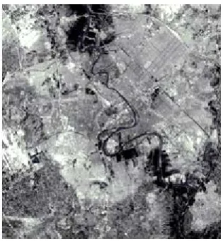
The multiband satellite image used in the classification was capture by Landsat satellite, it cover the area of
Baghdad city in Iraq. Figure (3) shows the six bands of used satellite image. The resolution of each band is
1024x1024 pixels, which carried acceptable range of informatic details about the image of consideration. One of
the most important factors of using the Landsat Baghdad image is the different concepts of landcover appears in
the image, which leads to different classes found in the image.
Figure3: The used six bands of Baghdad city given by Landsat.
The results of the dispersion coefficient (D) of used six bands are given in Table (1). It is shown that the greatest
three values of the dispersion coefficients are belong to the bands (1, 2, and 3) respectively. Therefore, to
compose these bands with each other for making one color image, it is assumed that the band (1) is stand for
green (G), band (2) is stand for red (R), and band (3) is stand for blue (B) in the RGB colored image. Figure (4)
shows the result of the composition process. Actually, the composed image enjoyed with more contrast and
more visual details.
22
Figure 4: Result of the image composition.
Image transform is used to enhance the satellite image by using equation (12). It is applied on the three color
components (R, G, and B) of the image, which leads to converting the image from three bands into one band is
better and suited for machine based analysis. The image preparation aimed to make the contrast of the
considered image is full. Full contrast is achieved when choosing the values of Min2 and Max2 to be 0-255 by
using equation (13). Figure (5) shows the result of transformed and prepared image.
Figure 5: Results of image transform and preparation.
5.1 Enrollment Results
The result of enrollment phase is a dataset stored in two dimensional array (A), the number of columns of this
array is equal to the number of classes, while the number of rows of this array is equal to the length of the class.
The length of the class is equal to the number of pixels contained in the image block, which can be determined
by product the width by height of the block. The results of the uniform image partitioning is shown in Figure
23
8 8 pixel. The blocks greater than BMax lead to confuse the classification results, whereas the blocks less than
BMin lead to poor image parts and no information may found in image blocks. The moment of each image block
was computed according to equation (21), the minimum and maximum resulted values of computed moment are
shown in Figure (7). It is noticeable that the minimum value of the moment is zero, while the maximum value is
808.9465. The zero value refers to empty blocks, which have no information in, while the maximum value refers
to much information found in that block. The application of the K-Means needs to set the range of expanding
the clusters along the moment scale. Therefore, the range between the maximum and minimum values of the
moment is 808.9465, which is divided into five (NC=5) of regions each of which extended by a maximum
distance is equal to (Dk=808.9465/5=161.7893 unit).
Figure 6: Result of uniform image partitioning (BMax=8 pixels).
Figure 7: Sample range of resulted moment values.
Finally, the dataset array A contains image blocks corresponding to the final centroids resulted from the
application of the K-Means, each of these blocks represents a one column in the dataset array A sequentially.
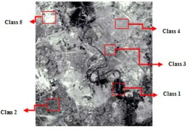
Figure (8) shows the behavior of these five columns that represent the labels of the discovered five classes of the
image under consideration, whereas Figure (9) displays the position of the image blocks that consisting in the
dataset array A. It is observed that dataset had contained different classes, which confirms the correct path of
24
depending on the details of each class.Figure 8: Behavior of five columns of five classes in the image.
Figure 9: Resulted five classes.
5.2 Classification Results
In the SVD method, the finding of best values of control parameters and the best partitioning of the quadtree is
very important problem since the control parameters govern the partitioning process that lead to intended
classification. Figure (10) shows the best control parameters of quadtree partitioning method.
25
Figure 11: Classified image using SVD method.
The classification result of the prepared image using the SVD method is displayed in Figure (11). It is shown
that the distribution of classes along the image region was acceptable. The best values of control parameters
make the partitioning process more accurate, which leads to accurate classification results. It seen that the
results of image partitioning based on image homogeneity measurements are very acceptable. The result of the
partitioning depends on the quantity of the uniformity for each block.
On the other hand, Figure (12) displays the classification result of the image using moment method (pixel-based
classification). The distribution of image classes along the image region is seems to be similar to that of the
block-based method. Also, it is noticeable that both methods were able to sense the small variation found in
some image regions, and truly classifying the fine details that regions.
Figure 12: Classified image using moment method.
5.3 Results Evaluation
To estimate the accuracy of the proposed two methods of satellite image classification, a standard image is
26
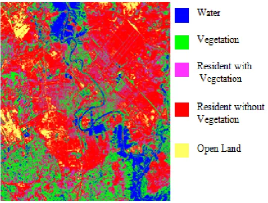
classified by Maximum Likelihood Method using ArcGIS software version 9.3. The classification map in this
image is shown in Figure (13), there are five distinct classes; they are: water, vegetation, residential with
vegetation (Resident -1), residential without vegetation (Resident -2), and open land, let we denote them as C1 for class water and C2 for class vegetation and C3, C4, C5 for classes Resident with vegetation, Resident without vegetation, and Open Land respectively.
The process of comparison was carried out pixel by pixel to guarantee the comparison result gave more realistic
indication. The procedure is done by counting the number of pixels in the classified image that gave identify
same class in the standard classified image. Then, the percent (PT) of the identical classified pixels (Cp) to the
total number of pixels (Tp) found in the image is computed as follows:
… (31)
Where, PT represents the overall accuracy (OA) of the proposed classification relative to the classification of the standard classified image given by GSC. Moreover, this relation can be employed to estimate the accuracy of
each class in the image separately. This is carried out by examining pixels of classified image that identify same
class in the standard classified image, which can be given in the following relation:
… (32)
Where, Pk is the classification accuracy of kth class that represents the user's accuracy (UA), Cc is the total number of pixels that classified as same as its corresponding pixels in the standard classified image given by
GSC, and Tk is the total number of pixels belong to the kth class in the classified image.
27
Accordingly, the producer accuracy (PA) can be computed using the following relation:
… (33)
Where, Pp represents the producer accuracy (PA), and Cp is the total number of pixels of each class in the standard classified image. The two parameters Pc and Pp are prepared to estimate both the commission error (EC) and omission error (EO) as follows:
EC = 100- PK … (34)
EO = 100- PP … (35)
The use of equation (31) on the whole image gives best estimation for pixel classification rather than the use of
random selected areas since the selection of small considered area may gave unstable result at each run of
comparison due to the change of position of considered area. The evaluation results of both SVD method (block
based classification) and moment method (pixel based classification) are listed in Tables (3 and 4) respectively,
these tables include the overall accuracy and class accuracy for the two adopted classification methods. Further
evaluation was indicated by measuring the area covered by each class using the following relations:
… (36)
… (37)
Where, represent the area covered by each class in both two adopted classification methods, and represent
the area covered by each pixel in standard classified image. Table (2) shows the area covered by each class for
the classified image mentioned before.
28
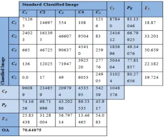
Table 3: The results of SVD classification method.
29
6.Results DiscussionThese results showed the classification methods were successful due to the percents of identical classes (Pk)
were acceptable. In SVD method, it is noticeable that the class of Resident with Vegetation (C3) has less identical percent due to the details of such class is large enough to be described in the used image, while the
class of water (C1) has a high identical percent due to it appeared in different spectral intensity in comparison with other classes, whereas; other classes are distributed moderately between the two mentioned classes. Also, it
showed that the overall accuracy of the classified satellite image is 70.64075%, while the total accuracy is about
81.83279% when the Resident without Vegetation (C4) and Resident with vegetation (C3) classes are regarded as same class. Figure (14) indicates that the class of C1 showed high identification percent in comparison with that of standard image relative to other classes in the standard image. Moreover, Table (3) mentioned that the
largest user's accuracy achieved with the high accuracy for the class of C1, the high value of user's accuracy has been found 81.13046 % for comparison between the results of the standard classified image and the SVD based
classified image, while the smallest user's accuracy was found in the class of Resident with Vegetation (C3) 49.34067%. It is concluded that the rest user's accuracy for the classes of satellite image are limited between the
maximum and minimum percent user's accuracy. On other hand, the high producer accuracy achieved for the
class C4 is 86.53535% and the smallest producer accuracy for the class C3 is 43.20286% the rest classes are limited between the larger and smaller producer accuracy as shown in Figure (15), where the class of Resident
with Vegetation has the smallest accuracy value. Also, Figure (16) describes the variation of each class in both
user's accuracy and producer accuracy, where the user's accuracy classes: water, resident With Vegetation, and
Open Land class are greater than their producer accuracy, while the user's accuracy of C2 and C4 are less than the producer accuracy of the standard classified image, which indicates the classes of C1, C2 and, C3 are more changed compared with the other classes.
In moment method, it is noticeable that the class of Open Land (C5) has less identical percent due to it was appeared very bright region in the used image, while the other classes have a high identical percent. Also, the
identical percent of moment method was better than that of SVD method because the later one depends on
classifying the image block by block, in which the minimum block size was 2 pixels, which may be relatively
large in comparison with the medium resolution of Landsat image. For this reason, the moment method showed
better results since it was going to classify the image pixel by pixel, which independent on the image resolution. Figure 14: Classes accuracy in SVD method.
0 0.1 0.2 0.3 0.4 0.5 0.6 0.7 0.8 0.91
C1 C2 C3 C4 C5
30
The results of moment method listed in Table (4) shows that the overall accuracy of the classification is 95.84%
due to the high user's accuracy and producer accuracy are yield. This make the omission and commission errors
are very small values as given in Table (4), the high identification percent of moment classification method are
for classes: C4, C1, C2 and C3 where the user accuracy are 100%, and user accuracy is 55.43% for class of C5, and producer accuracy of classes: C1, C2, C3 and C5 are 100%, while it is 90.38305% for the class of C4 in the standard classified image as shown in Figure (17). The user's accuracy of classes of Water, Vegetation, and
Resident with vegetation of the classified image are not changed, while the producer accuracy of the standard
classified image are relatively changed. The user's accuracy of the Open Land class is less than the producer
accuracy. Also, the user's accuracy of the Resident without vegetation class is greater than the producer
accuracy of the standard classified image. Figure (18) shows the user's accuracy of each class of moment
method, where the user accuracy of Open Land class is less than other classes, while the producer accuracy of
Resident without vegetation class is the least as shown in figure (19).
Figure 15: Producer accuracy of classes in SVD method.
Figure 16: Relation between producer and user's accuracy
of classes By using SVD Method.
Figure 17: Relation between producer and user's accuracy
31
Figure 18: User's accuracy of classes in Moment Method.
Figure 19: Producer accuracy of classes in Moment method.
7.Conclusions and Future Work
In this paper, the moment classification showed high accurate classification where, the identical percent of
moment classification method was better than that of SVD classification method. Where, the moment
classification method gave classification accuracy 95.84%, which is better than the SVD classification that gave
classification accuracy of about 81.5%. The classification results of moment classification method show that the
user's accuracy of classes: Water, Vegetation and Resident with vegetation classes are unchanged in comparison
with the producer accuracy, while the user's accuracy of Resident without vegetation is greater than the producer
accuracy for about 10%. Also, the user's accuracy of Open Land class is less than that of producer accuracy for
about 44.57%, which referred to the error commission. When using SVD method, the overall accuracy of the
classified satellite image is 70.64075%, which can be rised to be about 81.83279% when regarding both
Resident without vegetation and Resident with vegetation classes as same class. Where the used of quadtree
serves the classification stage due to the block size was smaller time by time till reaching to spectrally
homogenous region. And, the classification results of SVD method show that the variation of each class in both
user's accuracy and producer accuracy, where the user's accuracy classes: water, resident With Vegetation, and
Open Land class are greater than their producer accuracy, while the user's accuracy of Vegetation and Resident
without vegetation are less than the producer accuracy of the standard classified image, which indicates the
classes of water, Resident with vegetation and, Vegetation are more changed compared with the other classes.
32
present work, which help to achieve a higher level of performance efficiency, the most important suggestions
are given in the following:
1. Classify the satellite image by using Neural Network instead of Singular Value Decomposition as a
block based oriented method.
2. The use of genetic algorithm for classify satellite image instead of SVD method with K-Means
algorithm for enrollment phase to prepare dataset A.
3. Used ISO Data instead of K-Means for enrollment phase to prepare Dataset A with the moment of each
block.
4. It can be used Fuzzy c-means instead of K-Mean for enrollment phase to prepare Dataset A.
Acknowledgements
I would like to acknowledge my sincere thanks and appreciation to Dr. Mohammed S. Altaei for helping the
paper, assistance, encouragement, valuable advice, for giving me the major steps to go on to explore the subject,
sharing with me the ideas in my research and discuss the points that I left they are important. Grateful Thanks
are due to the Head of Computer Science Department, and the staff of the Department at College of Sciences of
Al-Nahrain University for their kind attention.
References
[1] Chijioke, G. E. " Satellite Remote Sensing Technology in Spatial Modeling Process: Technique and
Procedures", International Journal of Science and Technology, Vol. 2, No.5, P.309-315, May 2012,.
[2] Baboo, Capt. Dr.S S., and Thirunavukkarasu,"Image Segmentation using High Resolution
Multispectral Satellite Imagery implemented by FCM Clustering Techniques", IJCSI
International Journal of Computer Science Issues, ISSN (Print): 0814 | ISSN (Online):
1694-0784, vol. 11, Issue 3, no 1, S., May 2014.
[3] Sunitha A., and Suresh B. G., " Satellite Image Classification Methods and Techniques: A Review",
International Journal of Computer Applications, pp. 0975 – 8887, Volume 119 – No.8, June 2015.
[4] Mayank T., "Satellite Image Classification Using Neural Networks", International Conference:
Sciences of Electronic Technologies of Information and Telecommunications, 2005.
[5] Al-Ani L. A. and Al-Taei M. S.,"Multi-Band Image Classification Using Klt and Fractal
Classifier ", Journal of Al-Nahrain University Vol.14 (1), pp.171-178.
[6] Hameed M. A. Taghreed A. H., and Amaal J. H., 2011, " Satellite Images Unsupervised
Classification Using Two Methods Fast Otsu and K-means ", Baghdad Science Journal, Vol.8 (2) ,
33
[7] Bin, T.,Azimi-Sadjadi, M. R. Haar,T. H. V.Reinke, D., " Neural network-based cloud classification
on satellite imagery using textural features", IEEE, Vol. 3, p. 209 - 212, 1997.
[8] Márcio L. Gonçalves1, Márcio L.A. Netto, and José A.F. Costa, "A Three-Stage Approach Based on
the Self-organizing Map for Satellite Image Classification", Springer-Verlag Berlin Heidelberg, pp.
680–689, 2007.
[9] Sathya, P., and Malathi, L., "Classification and Segmentation in Satellite Imagery Using Back
Propagation Algorithm of ANN and K-Means Algorithm", International Journal of Machine
Learning and Computing, vol. 1, no. 4, October 2011.
[10] Rowayda, A. S.," SVD Based Image Processing Applications: State of The Art, Contributions and
Research Challenges", International Journal of Advanced Computer Science and Applications, Vol.3,
P.26-34.
[11] Bjorn F., Eric B., IreneWalde, Soren H., Christiane S., and Joachim D., 2013, "Land Cover
Classification of Satellite Images Using Contextual Information", ISPRS Annals of the
Photogrammetry, Remote Sensing and Spatial Information Sciences, Volume II-3/W1, 2012.
[12] Ankayarkanni and Ezil S. L., "A Technique for Classification of High Resolution Satellite Images
Using Object-Based Segmentation", Journal of Theoretical and Applied Information Technology,
Vol. 68, No.2, and ISSN: 1992-8645, 2014.
[13] Harikrishnan.R, and S. Poongodi, "Satellite Image Classification Based on Fuzzy with Cellular
Automata", International Journal of Electronics and Communication Engineering (SSRG-IJECE),
ISSN: 2348 – 8549, volume 2 Issue 3, March 2015.
[14] Akkacha B., Abdelhafid B., and Fethi T. B., "Multi Spectral Satellite Image Ensembles
Classification Combining k-means, LVQ and SVM Classification Techniques", Indian Society of
Remote Sensing, 2015.
[15] Thwe Z. P., Aung S. K., Hla M. T., " Classification of Cluster Area For satellite Image",
International Journal of Scientific & Technology Research Volume 4, Issue 06, 2015,.
[16] Anand, U.; Santosh, K. S. and Vipin, G.S., " Impact of features on classification accuracy of IRS
LISS-III images using artificial neural network ", International Journal of Application or Innovation
in Engineering and Management ,V. 3,P. 311-317, October 2014.
[17] Neil M., Lourenc M., and Herbst B. M.," Singular Value Decomposition, Eigenfaces, and 3D
Reconstructions", Society for Industrial and Applied Mathematics, Vol. 46, No. 3, pp. 518–545, 2004.
34
MRF Model", Journal of Network Communications and Emerging Technologies (JNCET), Volume 1,
Issue 1, 2015.
[19] Ranjith K. J., Thomas H. A., and Mark Stamp, "Singular value decomposition and metamorphic
detection", Springer-Verlag France, J Comput Virol Hack Tech, 2014.
[20] Ilya S., James M., George D., and Geoffrey H.," On the importance of initialization and
momentum in deep learning", International Conference on Ma-Chine Learning, Atlanta, Georgia,