The observation operational techniques used in satellite geodesy

(1)

The observation operational techniques used in

satellite geodesy

Milad Khosravi

1

_{, Reza Hemati}

1

_{, Ali Khodakarami Fard}

2*

_{and Mohammad Khosravi}

3

1- Department of Civil Engineering , Shahrood Branch, Islamic Azad University, Shahrood, Iran 2- Department Of Geology, Khorramabad Branch, Islamic Azad University, Khorramabad, Iran

3- Department Of Surveying, Nonprofit Institute of higher education Yassin Boroojerd, Iran

Corresponding author: Ali Khodakarami Fard

ABSTRACT: The observation techniques used in satellite geodesy can be subdivided in different ways. One possibility has been alrcady introduced in, namely a classification determined by the location of the observation platform

- Earth based techniques (ground station satellite), - satellite based techniques (satellite ground station), - inter-satellite techniques (satellite satellite).

Another classification follows from the observables in question. A summary of the most important operational techniques is given. References to the specific artificial satellites are included.

Keywords: observation, satellite, geodesy, platform, techniques.

INTRODUCTION

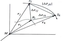
In this study a brief overview of the principal observation techniques, is given. The fundamental equation of satellite geodesy can be formulated as (see Fig 1.1) r S(t) = rB(t)+ ρ(t)

or

r j(t) = ri(t) + ∆ri j(t).

For a solution to equation (1.1) we have to establish a relation between the observations, characterized by the vector ∆ri j(t), and the Parameters which describe the satellite position rj(t) as well as the location of the observation

station ri(t). In the estimation process either all parameters can be treated as unknowns, or some of the parameters

are considered to be known, in order to stabilize and to simplify the solution. In general, a nonlinear observation equation model between the observations and the parameters is introduced:

(2)

1704

L + υ = Φ(X),

with

L the vector of the observations,

X the vector of the unknown parameters,

Φ a nonlinear vectorial function, and υ the vector of the residuals, containing the unmodeled components of the total estimation Process. The observation equation (1.2) can be linearized when approximate values Xo are

introduced for the unknown parameters. With

L0 = Φ(X0)

it follows that the vector of residual observations

l = L – L0 (1.3)

and the vector of residual parameters

x = X – X0. (1.4)

The linear form of (1.2) is then

l + υ = AX. (1.5)

The design matrix A contains the partial derivatives of the observations with respect to the parameters, developed around the approximate point of expansion X0:

𝐴 = (𝜕𝛷(𝑋)

𝜕𝑋 )0. (1.6)

The system of equations (1.5) can be solved in a least-squares adjustment process, based on the minimization of the function

υT _{Pυ minimum, (1.7)}

and yields a best estimate x of the unknown parameters. P denotes the weight matrix of the observations. For a full treatment of the subject see textbooks on adjustment or estimation techniques, for instance Wolf (I97S); Pelzer(1985); Koch (1990); Niemeier (2002). Textbooks with special emphasis on GPS techniques are Leick (1995) and Strang, Borre (1997)- The modern term estimation used in this book is equivalent to the classical term adjustment.

The parameters in equation (1.2) to (1.5) can be subdivided into different groups, for instance into:

(1) Parameters describing the geocentric motion of the observation station r B (t). The first of these are the

geocentric station coordinates. Then there are geodynamic parameters, describing the relation between the Earth-fixed terrestrial reference system and the space-Earth-fixed inertial reference system, namely the polar motion and Earth rotation parameters. Also belonging to this group are the parameters used for the modeling of solid Earth tides and tectonic crustal deformations. Finally, the transformation parameters between geocentric and particular geodetic or topocentric reference frames may be considered.

(2) Parameters describing the satellite motion rS(t). These are, besides the satellite coordinates, the harmonic

coefficients of Earth's gravity field, and parameters describing other gravitational or non-gravitational perturbations, like the solar radiation pressure.

(3) Parameters influencing directly the observations ρ(t). These are e.g. atmospheric parameters, clock parameters, and signal propagation delays.

It is obvious that a complete solution, where all parameters are determined simultaneously, cannot be obtained by simple means. Certain conditions, or requirements, have to be introduced in order to avoid a singularity of the equation system. The combined determination of coordinates and gravity potential coefficients is often called a satellite solution or only a solution; the product is named an Earth model.

In general only a few particular parameters or groups of parameters are of interest, and the other parameters are considered to be known values. The satellite orbit is often treated as known when the coordinates of the observation stations are to be estimated. For the determination of polar motion parameters and universal time, the coordinates of the control stations and Earth's gravity field are usually introduced from other solutions.

(3)

1705

Instead of estimating the parameters during the adjustment process, they can be eliminated through a suitable arrangement of observations. They are cancelled when simultaneous observations at different stations are different. This technique is often applied for the parameters of group(3). The satellite coordinates can also be eliminated, and need no longer be treated as unknown parameters, when observations are made simultaneously at a sufficiently large number of stations. The observation technique becomes more geometric in character. This geometrical concept of satellite geodesy was used particularly with camera observations.

Geometrical methods are by their nature relative methods, and they do not provide geocentric coordinates. This is why some problems in satellite geodesy cannot be solved with the geometrical methods.

Dynamical methods of satellite geodesy are used, when a force model is required for the description of the satellite motion. The orbit must either be known from external sources, for instance from an ephemeris service, or the orbit must be determined within the adjustment process, be it completely, or partially. Different concepts are in use.

When simultaneous observations are available from at least two stations, corrections to some particular orbital elements or "degrees of freedom" (up to six in number) can be estimated for a short portion of the orbit, together with the other adjustment parameters. This procedure is also called "adjustment with a relaxed orbit", or the semi-short-arc method. No particular forces acting on the satellite are considered in this technique; rather some of the degrees of freedom in the satellite orbit (orbital parameters) are eliminated via a geometric procedure.

A further step is that for a short portion of the orbit, based on a given force field, some orbital elements are estimated as parameters from the observations. This procedure is called the short-arc method. For even longer orbits, of several. revolutions, a larger number of perturbation parameters must be estimated (ef. Figure 2). The term for this technique is the long-arc method. The method is used e.g. for the parameter estimation of polar motion, Earth rotation, solid Earth tides, and the anomalous gravity field of Earth.

Figure 2. Role of the satellite orbit in the parameter estimation process

Long-arc methods are mostly used for the analysis of scientific problems. For operational tasks of applied satellite geodesy, the orbit is either taken as known, or a limited number of parameters are estimated for the orbit improvement within the adjustment process. For global radio navigation systems, like GPS, in general no orbit improvement is necessary because very precise orbits are available through particular services like the International GPS Service (IGS).

With observations from a single station the parameter estimation process is usually restricted to the determination of the station coordinates only. The number of parameters can be increased when simultaneous observations are available from several stations; corrections to the satellite orbit and observation biases may then be estimated.

For the solution of a general and global parameter estimation problem, observations to a large number of different satellites are required from many globally distributed stations. Figure 3 contains a schematic representation concerning the process of observation and parameter estimation.

Figure 3. Functional scheme for the use of satellite observations

Satellite observations Transform raw data into observations

Preprocessing Corrections for signal

propagation, time,elativity,

ambiguities, normal points

Computed values from observations

Parameter estimation

Numerical analysis, Geodesy, Orbital mechanics, Coordinate transformations

Station coordinates, Gravity field coefficients, Satellite positions, Polar motion, Earth rotation, Ocean and solid

Earth tides, Geodynamic parameters, Atmospheric parameters Observation biases

Estimation of aceuracy and reliability

Fixed orbit Semi Short Arc (relaxed orbit) Short Arc Long Arc

(4)

1706

RESULTS AND DISCUSSION

Discussion:

1.1 Determination of Directions

Photographical methods are almost exclusively used for the determination of directions. An artificial satellite which is illuminated by sunlight, by laser pulses, or by some internal flashing device, is photographed from the ground, together with the background stars. The observation station must be located in sufficient darkness on the night side of Earth. The stars and the satellite trajectory form images on a photographic plate or film in a suitable tracking camera, or on a CCD sensor. The photogram provides rectangular coordinates of stars and satellite positions in the image plane, which can be transformed into topocentric directions between the observation station and the satellite, expressed in the reference system of the star catalog (equatorial system, CIS).

Two directions, measured at the same epoch from the endpoints of a given base line between observing stations, define a plane in space whose orientation can be determined from the direction cosines of the rays. This plane contains the two ground stations and the simultaneously observed satellite position. The intersection of two or more such planes, defined by different satellite positions, yields inter station vector between the two participating groundstations (Figure 4). When more stations are involved, this leads to regional, continental, or global networks. Note that these networks are purely geometric.

Direction measurements have also been used for orbit determination, and they were introduced into early comprehensive solutions for Earth models (gravity field coefficients and geocentric coordinates). Some satellites are equipped with laser-reflectors. In such cases the directions and ranges can be determined simultaneously, and provide immediately the vector ρ(r) between the ground station and the satellite.

Figure 4. The use of directions with satellite cameras

Initially passive balloon satellites were used as targets, such as the first experimental telecommunication satellites, ECHo-1 and ECHO-2. In 1966 a dedicated geodetic balloon satellite, PAGEOS (PAssive GEOdetic satellite), with a diameter of 30 m was launched for the observation of the BC4 world Network. The satellite was placed into an orbit of about 3000 to 5000 km altitude and was used for about six years. Today, laser pulses can be reflected by satellites equipped with corner cube reflectors, and be used for the determination of precise directions. However, the achievable accuracy is very low when compared with modern ranging methods. This is why today the measurement of directions only plays a minor roll in satellite geodesy.

A certain revival took place with the launch of the Japanese Geodetic satellite AJISAI in 1986 (Sasaki, 1983; Komaki ., 1985), A modern application is the use of powerful CCD-techniques for the directional observation of geostationary satellites.

Directional information can also be derived by analysis of electromagnetic signals transmitted from a satellite. The related techniques, which have been realized so far, yield only a rather low accuracy. very Long Baseline Interferometry (VLBI), on the other hand, is one of the most accurate observation techniques in geodesy, and provides precise directions to extragalactic radio sources. The application of the VLBI technique using radio signals from artificial satellites is under discussion

1.2 Determination of Ranges

For the determination of distances in satellite geodesy the propagation time of an electromagnetic signal between a ground station and a satellite is measured. According to the specific portion of the electromagnetic spectrum we distinguish between optical systems and radar systems.

(5)

1707

We distinguish the one-way mode and the two-way mode. In the two-way mode the signal propagation time is measured by the observer's clock. The transmitter at the observation station emits an impulse at epoch tj. The impulse

is reflected by the satellite at epoch tj + Δtj, and returns to the observation station where it is received at epoch tj +

Δt'

j. The basic observable is the total signal propagation time Δtj. Without considering relativistic effects, we

find Δtj = 2 Δt'j

Following Figure 5 with c being the signal propagation velocity, we obtain the basic equation for the distance measurement in the two-way mode:

|rj− ri| = |∆rij| = 1

2c. ∆tj (1.8)

One typical example for this mode is the Satellite Laser Ranging (SLR) tech nique. The observer,_{s clock can}

also be placed in the satellite, e.g. for space borne laser, or radio systems like PRARE.

Figure 5. Concept of range measurements to satellites

In the one-way mode we assume that either the clocks in the satellite and in the ground receiver are synchronized with each other, or that a remaining synchronization error can be determined through the observation technique. This is, for instance, the case with the Global Positioning System (GPS) W. Equation (1.8) simplifies to

|∆rij| = c. ∆tj (1.9)

Further we distinguish between either impulse or phase comparison methods. when a clear impulse can be identified, as is the case in satellite laser ranging, the distance is calculated from the signal propagation time using equation(1.8).

With the Phase comparison method, the phase of the carrier wave is used as the observable.In the two- way mode the phase of the outgoing wave is compared with the phase of the incoming wave. In the one-way mode the phase of the incoming wave is compared with the phase of a reference signal generated within the receiver In both cases the observed phase difference, ΔΦ, corresponds to the residual portion, Δλ, of a complete wavelength. The total number, N, of complete waves between the observer and the satellite is at first unknown. This is the ambiguity problem. The corresponding equation in the two-way mode is

|∆rij| = 1

2(∆λ + Nλ). (1.10)

The factor 1

2 disappears in the one-way mode. Different methods are used for the solution of the ambiguity term

N, for example:

- measurements with different frequencies (e.g. SECOR),

- determination of approximate ranges with an accuracy better than λ/2 (e.g. GPS with code and carrier Phases),

- use of the changing satellite geometry with time (e.g. GPS carrier phase observations), - ambiguity search functions (e.g. GPS),

and phase comparison methods also show differences with respect to the signal propagation in the high atmosphere. Distances derived from phase measurements depend on the phase velocity υP of the particular

frequency, whereas distances derived from impulse measurements are based on the respective group velocity υg.

The ionosphere is a dispersive medium, and hence the phase velocity is greater than the group velocity.

Distinct satellites are used for the different methods of range measurements. For satellite laser ranging (SLR) the satellites are equipped with suitable reflectors. Dedicated laser satellites are for example LAGEOS-1,2 (LAser GEOdynamic Satellite; orbital height about 5900 km), STARLETTE and STELLA (orbital height about 800km). There are now about 70 satellites equipped with laser reflectors.

(6)

1708

simultaneously between three known ground stations and at least three different satellites the unknown coordinates of a station relative to the stations whose coordinates are known can be derived. This procedure has been used on a regular basis with the SBCOR System, and it can also be used in satellite laser ranging (SLR) under favorable atmospheric conditions. Similarly, the unknown coordinates of ground stations can be derived from three satellites whose positions are known in the two-way mode, and from four satellites whose positions are known in the one-way mode.

In many cases the often high data rate of range observations, (e.g. one observation per second) is not required in the subsequent analysis process. The data are hence compressed to so-called normal points. For details of normal point generation see.

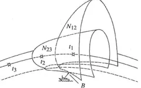
1.3 Determination of Range Differences (Doppler method)

Fig1.6 illustrates the geometrical principle of position determination from range differences between one observer and two pairs of satellite positions. The satellite positions at epochs tl, t2 and t3 are taken as known. Each

of the observed range differences (Bt1 - Bt2) and (Bt2 Bt3) define a hyperbolic surface in three dimensional space.

The observer (e.g.on a ship) is situated at the intersection of the hyperbolic surfaces with Earth,_{s surface. It becomes}

evident from geometrical considerations that with a single satellite pass only a two dimensional position can be determined. For a three-dimensional solution several satellite passes are required.

Figure 6. Geometrical interpretation of the positioning with range-differences

The range differences are derived from the measurement of the frequency shift caused by he change of range between the observer and the satellite during a given satellite pass. The satellite transmits a signal of known frequency fswhich is tracked by a ground receiver. The relative motion ds / dt between the receiver and the transmitter

causes the received frequency fr (t) to vary with time as

fr(t) = fs(1 − 1 c

ds

dt). (1.11)

This is the well-known Doppler effect. The frequency shift in a given time interval tj, tk is observed, and is scaled

into a range difference Δrijk (cf. Fig1.5) The related observation equation is

|rk− ri| − |rj− ri| = |∆rik| − |∆rij| = |∆rijk|. (1.12)

The observation of the Doppler effect is frequently used in satellite geodesy. The technique is always applicable when a satellite, or a ground-beacon, transmits on a stable frequency. The orbital elements of the very first satellites were determined by observing the Doppler-shift of the satellite signals. The most important application of the Doppler method in geodesy has been with the Navy Navigation Satellite System (TRANSIT). A current space system based on the Doppler technique is DORIS.

The Doppler effect can also be used for the high precision determination of range rates |∆rjk| between satellites.

This method is named Satellite-to-Satellite Tracking (SST), and it can be applied to the mapping of a high resolution Earth gravity field

1.4 Satellite Altimetry

This is a specific form of ranging, where the vertical distance between a satellite and Earth,_{s surface, in particular}

(7)

1709

from the satellite and reflected from the sea surface. The data are communicated in a suitable way from the satellite to the user.

With a knowledge of the satellite orbit, the satellite altitude, h, above the Earth ellipsoid is also known and provides via the simplified relation

M = h – a0 (1.13)

The separation M between the mean sea level and the ellipsoid (Fig1.7). M approximately equals the geoid height; hence satellite altimetry can be used to determine the geoid over the oceans. A more sophisticated evaluation requires some corrections, in particular to model the separation between the instantaneous sea surface and the geoid, and to model the deviations between the true satellite trajectory and the computed orbit.

GEOS-3 and SEASAT-l were the first two satellites to carry radar altimeters and have been used extensively for geodetic purposes. Further altimeter satellites were GEOSAT, ERS-l, ERS-2, TOPEX/POSEIDON, GFO, JASON and ENVISAT, providing significant contributions to geodesy, geophysics, and oceanography.

Figure 7 Simplified principle of satellite altimetry

1.5 Determination of Ranges and Range-Rates (Satellite-to-Satellite Tracking)

This method can be used for mapping the high frequency components of Earth,_s

gravity field. The observables are the range and the range rate, i.e. the relative velocity between two satellites. Different concepts have been proposed and are already realized or at the stage of realization. In the low-high configuration a low orbiting satellite (LEO, a few hundreds of kilometers orbital altitude) is combined with a satellite in a high (e.g, MEO or GEO) orbit, The advantage is that a rather long trajectory of the low orbiting satellite, which is particularly affected by high frequency components of the terrestrial gravity field, can be "seen" from the high orbiting satellite (Fig1.8). One example is CHAMP with GPS.

In the low-low configuration two satellites occupy the same low-altitude orbit separated by 100 to 300 km. A higher resolution of the gravity field is expected with this technique. The low-low configuration is used with GRACE.

Figure 8. Principle of satellite-to-satellite tracking, high-low and low-low configuration

1.6 Interferometric Measurements

The basic principle of interferometric observations is shown in Figure 9. A1 and A2 are antennas for the signal

reception. When the distance to the satellite S is very large compared with the baseline length b, the directions to S from A1 and A2 can be considered to be parallel. From geometric relations we obtain

d = A̅̅̅̅̅ = b. cosθ.1P (1.14)

(8)

1710

The observed phase difference is uniquely determined only as a fraction of one wavelength; a certain multiple, N, of whole wavelengths has to be added in order to transform the observed phase difference Φ into the range difference d. The basic in terferometric observation equation is hence

d = b. cosθ = 1

2πΦλ + Nλ. (1.15)

Figure 9. Interferometric measurements

The interferometric principle can be realized through observation techniques in very different ways. Equation (1.15) contains different quantities which can be used as derived observables, namely.

- the baseline length b between the two antennas,

- the residual distance d between the antenna and the satellite, and - the angle θ between the antenna baseline and the satellite.

In each case it is necessary to know, or to determine, the integer ambiguity term N. The determination is possible through a particular configuration of the ground antennas, through observations at different frequencies, or through well defined observation strategies. One example for the determination of directions to satellites by interferometric measurements is with the classical Minitrack - System, where the individual antenna elements are connected with cables. The achievable accuracy, however, is not sufficient for modem requirements in satellite geodesy.

With increasing baseline lengths the antennas cannot be connected directly with cables. The phase comparison between the antennas must then be supported by the use of very precise oscillators (atomic frequency standards). This is, for instance, the case with the Very Long Baseline Interferometry (VLBI) concept.

When natural radio sources (e.g. quasars) are observed with the VLBI technique, the range difference d is not determined through methods of phase comparison, but by the correlation of the signals obtained at both antennas. The signal streams are registered together with precise timing signals at both antenna positions, and they are later shifted, one against the other, within a correlator, until the maximum correlation is obtained. The time delay τ corresponds to the signal travel time between P and A1, and can be scaled to a range difference

d = τ· c. (1.16)

When artificial Earth satellites are used in the VLBI technique, .it cannot be assumed that the directions from the antennas to the satellites are parallel. Instead, the real geometry has to be introduced by geometric corrections; e.g. the wavefronts must be treated as curved lines.

The interferometric principle has been widely used in the geodetic application of the GPS signals. Both methods described above for the determination of the range.

Differences d are possible:

(a) The signals from the GPS satellites can be recorded at both antenna sites without any a priori knowledge of the signal structure, and later correlated for the determination of the time delay τ. A very large instrumental and computational effort is required, so the method is not really suitable for operational applications. It is, however, used to some extent in modem GPS receiver technology, in order to access the full wavelength of L2 under "Anti-Spoofing" (A-S) conditions.

(b) The phase of the carrier signal at both antenna sites can be compared, and the difference formed. These so called single phase differences can be treated as the primary observables. The method is now widely used forprocessing GPS observations.

(9)

1711

CONCLUSION

Besides the observables and observation techniques mentioned other methods were proposed, or are still in use, or are planned for forthcoming satellite missions. In many cases combinations of different observables are employed. One of the concepts proposed and now under development is satellite gradiometry. A gravity gra- diometer measures directly the second derivatives of Earth,_{s gravitational potential. It is very hard to achieve the required}

resolution with the available instrumentation. The same is true for the application of accelerometers in the satellite. A first mission based on this concept will be GOCE, planned for launch in 2006.

Earth observation satellites or remote sensing satellites carry a large quantity of sensors for the optical and microwave frequency domain. Of particular interest to geodetic applications is the Interferometric Radar (InSAR) technique which can be used to detect small deformations of Earth,_{s crust.}

REFERENCES

Gunter S. 2003. satellite geodesy, 2nd_{completely and extended edition, Berlin, New York pp. 134–152.}

http://www.iau.org/

http://hpiers.obspm.fr/icrs-pc/icrf/icrf.html

http://www.iers.org/IERS/EN/Home/home_node.html http://igscb.jpl.nasa.gov/

http://www.gaithersburgmd.gov/about-gaithersburg/city-facilities/international-latitude-observatory http://adsabs.harvard.edu/full/2000ASPC..208..147Y

http://www.ngs.noaa.gov/PUBS_LIB/Geodesy4Layman/TR80003D.HTM http://www.scopus.com/