© 2017 IJSRSET | Volume 3 | Issue 8 | Print ISSN: 2395-1990 | Online ISSN : 2394-4099 Themed Section: Engineering and Technology
Continuous Genetic Algorithm : A Robust Method to Solve
Higher Order Non-Linear Boundary Value Problem
Kavindra Soni, Dr. Mahendra Singh Khidiya
Department of Mechanical Engineering, College of Technology and Engineering, MPUAT, Udaipur, India
ABSTRACT
The aim of this work is to find the solution of linear and nonlinear boundary value problem using genetic algorithm. A continuous genetic algorithm has been design and applied to the solution of fourth-order nonlinear boundary value problem. The genetic algorithm solves the differential equation by a process of evaluating the best fittest solutions curve from a family of randomly generated solution curves. This method is applicable to both the linear and nonlinear differential equation of fourth-order. Numerical results presented in the work illustrate the applicability of the genetic algorithm for fourth-order linear and nonlinear boundary value problem.
Keywords : Genetic Algorithm, Fourth-Order Nonlinear Differential Equation, Centre-Difference Formula, Electrostatically Microcantilever Beam
I.
INTRODUCTION
Most fundamental laws of science are based on models that explain variation in physical properties and state of system described by differential equations. To find the solution of differential equation is difficult job. The difficulty is increase as the order of differential equation and nonlinearity is increase. Therefore, solving the nonlinear differential equation is perhaps the most difficult problem in all of numerical computation.
The work presented in this paper is motivated by the success of using continuous genetic algorithm for solution of second-order, two-point linear and nonlinear boundary value problems. Although there are many possible methods or techniques are available for solving linear and nonlinear differential equation problems, such as, finite element method, soothing method, Ritz energy technique, etc. but they are difficult to implement or they required some more advanced mathematical tools. That tools are may be root finding technique or solution of some initial value problem. While switching from linear to nonlinear problem, they also required any modification.
1.1 Differential equation
A differential equation is an equation where the unknown is a function and both the function and its
derivatives may appear in the equation. Differential equations are essential in the description of nature by physics. The central part of many physical theories is a differential equation: Newton’s and Lagrange equations for classical mechanics, Maxwell’s equations for classical electromagnetism, Schrodinger’s equation for quantum mechanics, Einstein’s equation for the general theory of gravitation. In addition, a problem occurs in the field of engineering and science such as electric power generation, optimization and path-planning application. Many of these problems are in the form of higher order differential equation.
nonlinear equation introduced by Kare et al [5]. Raudensky et al [6] present a genetic algorithm for solving the one-dimensional inverse heat conduction problem. A novel method based on continuous genetic algorithm is introduced by Z. S. Abo-hammour et al [7] for the solution of the second-order, two-point boundary value problem. Advanced continuous genetic algorithm and their application in the motion planning of robotic manipulators are proposed by Z. S. Abo-Hammour et al [8]. A numeric genetic algorithm is introduced by Cong P. Li T. [9]. M. W. Gutowski proposed a smooth genetic algorithm [10] applied for finding the distribution of magnetic nanocrystallites.
1.2 Genetic algorithm
Genetic algorithm (GAs) is stochastic population-based search techniques. GAs operates on a population of potential solutions applying the principal of survival of the fittest to produce better approximation to a solution. The appeal of GAs comes from their simplicity and robustness as well as their power to discover good solutions for complex high dimensional global optimization problems that are very difficult to handle by more conventional techniques (Forrest and Mitchell, 1993). They have performed well in a number of diverse application such as the solution of ordinary differential equations [3], solution to system of nonlinear equations [5], application of genetic algorithm and CFD for flow control optimization [11], collision-free Cartesian path planning of robot manipulation [12], numerical solution of boundary value problem [7].
The genetic algorithm is based on the triangle of genetic reproduction, evaluation and selection [13]. Genetic reproduction is performed by two genetic operators: crossover and mutation. Evaluation is performed by fitness function and selection is based on relative fitness.
1.3 Electrostatically microcantilever beam
Now a day wide range of research is going on the micro-electro mechanical system. The geometry of micro-actuator influences the mechanical stiffness and electrostatic force distribution. Electrostatically actuated microdevices are mostly susceptible due to an operational instability. A novel closed-form empirical relation to predict the static pull-in parameters of electrostatically actuated microcantilevers having linear width variation proposed by M. M. Joglekar and D. N.
Pawaskar [14]. Static and dynamic analysis of electrostatically actuated microcantilever using the spectral element method is proposed by P. V. Dileesh, S. S. Kulkarni, D. N. Pawaskar [15].
II.
METHODS AND MATERIAL
2.1 Continuous genetic algorithm
The solution curves of boundary value problems are smooth in nature. So, continuous genetic algorithm is used in this work. The construction of a genetic algorithm is based on the following conditions-
1. The genetic representation of potential problem solution,
2. A method for creating initial population of solution, 3. The design of the genetic operators,
4. The definition of the fitness function, 5. The setting of system parameters
Each of the above components greatly affects the solution obtained as well as the performance of the genetic algorithm. The genetic operators that are use in this work are describing below.
2.1.1 Initialization
The implementation of a genetic algorithm starts with generating a population of possible solutions. For the solution of boundary value problem the initialization function is smooth and it should satisfied the given boundary values. Two smooth initialization function: the Gaussian function and the tangent hyperbolic function are used [7].
2.1.1.1 Tangent hyperbolic function
The tangent hyperbolic function is used in this work is given below. This function has some limitation for a particular type of boundary condition. If the nodal values of the extreme end are same, it will not work. In that case, the Gaussian function is applied, which is described in next section.
( ( ))
Where P(i,j) is the value of the ith node for the jth parent.
µ is a random number within the range [11/4, 33/4] and it specified the centre of the function, σ is a random number within the range [1, 11/3] and it specifies the degree of dispersion [7]. Np is the number of initial population. The convergence speed is depending on the initialization function. If the initialization is closer to the final solution the convergence speed is faster and from study it is seen that after few generations convergence speed is governed by the selection, crossover and mutation operators.
2.1.1.2 Gaussian function
The Gaussian function which is used in this work for special boundary condition, is given as [7]
( )
For all 1 ≤ i ≤ N and 1 ≤ j ≤ Np
Where P(i,j) is the value of the ith node for the jth parent,
µ is a random number within the range [11/4, 33/4] and it specified the centre of the function, σ is a random number within the range [1, 11/3].
2.1.2 Evaluation
Evaluation is performed by the mean of fitness function. It is a measure of quality of the individual in the population. The fitness function is defined as
And R is overall residual. The main goal of the genetic algorithm is maximize the fitness function F.
2.1.3 Selection
The population is arranged in ascending order based on their relative fitness function value. The selection of population is rank based. The maximum fitness function values have highest rank and minimum fitness function values have lowest value. The bottom 50% of the population is discarded and the remaining 50% are selected for reproduction. The overall quality of the population is depending on the selection mechanism and its increase from one generation to the next.
2.1.4 Crossover
Crossover is the genetic algorithm operator that attempts to mix each pair of population selected as parents, to create the likelihood of keeping the good properties of each parent population in the offspring children [7]. Crossover provides the means by which valuable information is shared among the population. Crossover operator is implemented in several works in the literature. In this work crossover operator is expressed as
( )
( ( ))
For all 1 ≤ i ≤ N
Where P(i,j), P(i,k), CL and CL+1 represent the two
parents chosen from the mating pool and the two children obtained through crossover operator respectively, w represent the crossover weighting function within the range [1, 11/3]. The crossover operator also maintains the smoothness of the solution curves.
2.1.5 Mutation
Mutation operator has two important roles during the evaluation process in a genetic algorithm. First is to introduce unexplored genetic material to the population. Second is to maintain the diversity of the candidate solution in a population over the generations, preventing premature convergence of the genetic algorithm to suboptimal solution [7]. In this work mutation operator is expressed as
(
)
For all 1 ≤ i ≤ N, 1 ≤ j ≤ Np
Where C(i,j) represent the jth child produced through the crossover process, is the mutated jth child, M is the Gaussian mutation function and d represent a random number within the range [-1,1].
After evaluation process, the population is going to change in every generation because of the crossover and mutation operators. Due to this the best information or population is vanish. To overcome that problem elitism operator is applied. Elitism operator insures that in the next generation the best-fitted individual is not less than previous fitted individual.
2.1.7 Extinction and immigration operator
After few numbers of generations, the population is going to stagnate, due to repetitions of the crossover and mutation operator. To overcome this problem extinction and immigration operator is applied to the population. In this process, half of the population is generated by same initial population function [7]. The another half population is generated by this formula that is given as
For Np/2+1 ≤ j ≤ Np
Where P(i,j) is the jth parent generated by above operator,
P(i,1) represent the best fitted population, M and d has already described in previous section.
2.1.8 Scaling operator
For solving fourth-order linear and nonlinear boundary value problem by genetic algorithm, after few number of generations the shape of the curve is generated but the exact solution is far away. To generating exact solution scaling operator is introduce. This operator is given as
For all 1 ≤ i ≤ N and 1 ≤ j ≤ Np
Where is the jth parent generated by scaling operator, represent the previous generated population and is a random number between Fmax and 1. Fmax is the maximum value of fitness function so far found during the evaluation process.
2.1.9 Replacement
After the application of genetic operators to the initial (parent) population, a new population is generated. The previous population is replaced by new generated population, which is better fitted. This is also known as “life cycle” of the population.
2.1.10 Termination
The process described is iterated until an acceptable solution is found. The termination criterion is defined by the user, it could be either the difference in fitness value of few subsequent generations or a fixed number of generations which the user thinks, would provide a reasonable acceptable solution. In this work, the maximum fitness value is set to be 0.99999 and the maximum number of generation is set to be 500000. The genetic algorithm is terminating when one of the above criterion is met.
III.
RESULTS AND DISCUSSION
3.1 Problem formulation and numerical results
Genetic algorithm and its operators are described previous are coded in MATLAB (R 2011a) for the solution of boundary value problem. In problem formulation, there are two types of parameter, one is genetic algorithm related and another is boundary value related. These parameters are described in next section. After that, the numerical results are shown in graphical and tabular form.
3.2 Genetic algorithm related parameter
In this work, following parameters are used in each problem. The initial population size (Np) is set to be 100. The selection mechanism is rank based. The crossover and mutation probability is set to be 0.5 and 0.4 respectively. The number of elite parents, which are directly goes to next generation without any applications of genetic operators, is set to be 10. The value of δ is very from problem to problem. The scaling, extinction and immigration operator is alternatively applied after every 100 number of generations.
The genetic algorithm is stopped when one of the following conditions is satisfied. These are as following-
1. When the value of maximum fitness (Fmax) is reach to 0.99999.
2. When the number of generation is, exceed by 500000.
Genetic algorithm does not require information of derivatives, because it is an optimization tool. Due to this, the governing differential equation is converting into discretization form. The centred-difference formulas, with truncation error of order 0 (h2) is used to convert differential equation into discretization form.
As shown in the chapter 1, the general fourth-order differential equation two-point boundary value problem of the form
A ≤ x ≤ B
Together with boundary conditions
i. y(A)=a y (A)=b y″(B)=c y‴(B)=d ii. y(A)=a y″(A)=b y(B)=c
y″(B)=d
For the approximation, each derivative term is replaced in the discretized form by a difference quotient. The interval of the boundary value problem is equally partitioned into N+1 subinterval. The length of each subinterval is given as
Where N = 9 is a number of interior nodes.
For approximating y (xi), y″(xi), y‴(xi) and y‴ (xi) , the centre-difference formula is given as
With the help of above equation the original differential equation is rewrite in discretized form as follows:
The residual of ith node ( ) and the overall individual residual (R) is given as
√∑
To convert the minimization problem of R into a maximization problem of F a mapping of the individual residual R is required. Therefore, the fitness function is defined as
The maximization of above fitness function is the main task of genetic algorithm. The boundary value related parameters are as follows:
1. The number of interior nodes (N = 9). 2. The step size (h = 0.1).
3. The boundary conditions at both the ends that are vary from problem to problem.
4. The interval between which the differential equation is solved (0 ≤ x ≤ 1).
3.4 Numerical results
3.4.1 Case-1
Euler-Bernoulli beam equation is solving to find the deflection of a beam. In this case, one end of the beam is fixed and another end is free as shown in figure 4.1.
0 ≤ x ≤ 1
With following boundary condition
y (0)=0 y (0)=0 y″ (0)=0 y‴ (0)=0
where: E = Modulus of Elasticity (material property)
I = Moment of Inertia (geometry of material)
f(x) = load per unit length
y(x) = deflection (displacement) from vertical
L = length of the beam
L
f(x)
x = 0 x =1
x
Fig. 3.1 Cantilever beam with uniformly distributed load
The discretization form of above governing differential equation is given as
(
)
To find the exact information of any point we need information of four other points in centre-difference method. In this case, the value of node number 1 is known and all other all unknown.
Fig. 3.2 Cantilever beam with discretization
For nodes 2 to 11 information is generated initially by tangent hyperbolic function and for the information of nodes 0, 12 and 13 is founded by the help of given boundary conditions. For getting the information of any node by centre-difference formula, the information of four other nodes is needed.
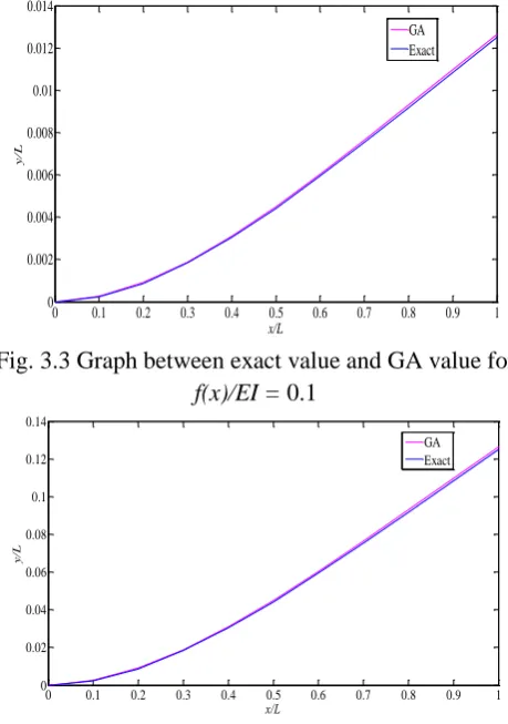
For example, for getting the information of node number 2, the information of node 0, 1, 3 and 4 is needed. But the genetic algorithm is only generating the information of 2 to 11 number of nodes. To overcome this problem the given boundary conditions are also convert into discretization form. The boundary condition in discretization form is give additional information for the solution curve. The genetic algorithm is coded in MATLAB (R 2011a) and the numerical results are compared with exact solution. These results are shown for f(x)/EI = 0.1 and 1 in figure 3.3 and 3.4 respectively.
Fig. 3.3 Graph between exact value and GA value for
f(x)/EI = 0.1
Fig. 3.4 Graph between exact value and GA value for
f(x)/EI = 1
Table 3.1 Comparison between exact and GA value for case-1.
f(x)/EI 0.1 1
Node (i)
Exact GA Exact GA
1 0 0 0 0
2 0.00023 0.00025 0.0023 0.0025
3 0.00087 0.00090 0.0087 0.0090
4 0.00183 0.00188 0.0183 0.0188
5 0.00304 0.00310 0.0304 0.0310
6 0.00442 0.00450 0.0442 0.0451
7 0.00594 0.00603 0.0594 0.0603 8 0.00753 0.00764 0.0753 0.0764
9 0.00917 0.00930 0.0917 0.0930
10 0.01083 0.01097 0.1083 0.1097
11 0.01250 0.01265 0.1250 0.1265
Fitness 0.99999 0.99999
In given loading value the genetic algorithm terminated before it reached the maximum number of generation (500000). The fitness function reached the maximum fitness value of 0.99999.
0 0.1 0.2 0.3 0.4 0.5 0.6 0.7 0.8 0.9 1 0
0.002 0.004 0.006 0.008 0.01 0.012 0.014
x/L
y/
L
GA Exact
0 0.1 0.2 0.3 0.4 0.5 0.6 0.7 0.8 0.9 1 0
0.02 0.04 0.06 0.08 0.1 0.12 0.14
x/L
y/
L
GA Exact
Imaginary node
use y′(x = 0) = 0
given
y(x = 0)= 0
use
y″(x = 1)= 0
x (m)
y
(
m)
3.4.2 Case-2
In this case, the genetic algorithm is used to numerically approximate the deflection of electrostatically actuated microcantilevers beam which is shown in figure 3.5. The governing differential equation in dimensionless form is given as [14].
( )
(
)
And the four dimensionless boundary condition are expressed as
|
| | |
Where w(x) = 1-fx is the dimensionless width function,
is the fringe parameter,
is the voltage in dimensionless form, E = the effective young’s modulus,
L = the length of the microcantilever beam, = width of the cantilever at the fixed end, = initial gap between the two electrodes,
v = potential difference between the two electrodes,
H = thickness of the cantilever beam.
But in this case prismatic microcantilever beam is solved. For this the equation is derived for no width variation so, the modified governing differential equation is expressed by equation and figure 3.5 show the schematic of an electrostatically actuated prismatic microcantilever beam.
Fig. 3.5 Schematic of an electrostatically actuated prismatic microcantilever beam (adapted from [14]).
( ) (
)
With the help of centre-difference formula the equation (4.15) is converted into discretization form, which is given as
(
)
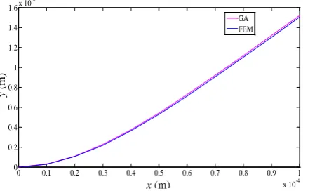
With the help of equation above the genetic algorithm solves the fourth-order nonlinear boundary value problem. The final results are shown in graphical and tabular form which is shown in figure 3.6 and 3.7 and table 3.2 respectively.
Fig. 4.18 Graph between FEM value and GA value for v
= 1 V
Table 3.2 Comparison between FEM and GA value for case-3.
v (volt) 1 10
Node (i) FEM (x 10-9)
GA (x 10-9)
FEM (x 10-7)
GA (x 10-7)
1 0 0 0 0
2 0.002689 0.002953 0.002737 0.003005
3 0.010182 0.010690 0.010366 0.010885
4 0.021475 0.022209 0.021870 0.022622
5 0.035686 0.036623 0.036351 0.037316
6 0.052046 0.053165 0.053029 0.054186
7 0.069907 0.071184 0.071244 0.072569
8 0.088739 0.090148 0.090453 0.091921
9 0.108130 0.109645 0.110234 0.111820
10 0.127783 0.129378 0.130286 0.131961
11 0.147522 0.149170 0.150426 0.152164
Fitness 0.99999 0.99999
In this case the FEM solution is also obtain from MATLAB (R 2011a) and code is referred from Static
0 0.1 0.2 0.3 0.4 0.5 0.6 0.7 0.8 0.9 1 x 10⁻⁴ 0
0.5 1 1.5x 10
-10
y
(
m)
x (m)
and dynamic analysis of electrostatically actuated microcantilever using the spectral element method [15].
It’s observed from the graph and tabular data that the GA solution is closely match with the FEM solution. The genetic algorithm is applicable for both linear and nonlinear fourth-order boundary value problems.
Fig. 3.7 Graph between FEM value and GA value for v
= 10 V
IV.
CONCLUSION
The fourth-order linear and nonlinear boundary value problems are successfully solved by genetic algorithm. Genetic algorithm uses the objective function information and not the derivative information. Diversity is essential to the genetic algorithm because it enables the algorithm to search a large region of the population. For the solution of boundary value problem the solution curve must be smooth in nature. The genetic algorithm is versatile in nature because the operators of genetic algorithm are user and problem dependent and easy to excess. Genetic algorithm is applicable to both linear and nonlinear case without any fail. The numerical results from genetic algorithm are closely matched with available results.
V.
FUTURE SCOPE
In this work the static problem is solved for nonlinear fourth-order differential equation. In future, this method can be used for dynamic fourth-order differential equation. The present method, finds the deflection of the prismatic microcantilever beam under varying potential difference. Further, this method can be applied for finding the deflection of triangular microcantilever beam under varying potential difference.
VI.
REFERENCES
[1]. Pryor RJ, Using a genetic algorithm to solve fluid flow problems. Transactions of the American Nuclear Society 1990; 61:435.
[2]. Pryor RJ, Cline DD. Use of a genetic algorithm to solve two-phase fluid flow problems on an Ncube multiprocessor computer. SAND92-2847C, Sandia National Laboratories, 1992.
[3]. Diver DA, Applications of genetic algorithms to the solution of ordinary differential equations. Journal of Physics A Mathematical and General 1993; 26(14):3503-3513.
[4]. Chaudhury P, Bhattacharyya SP, Numerical solutions of the Schrodinger equation directly or perturbatively by a genetic algorithm: test cases. Chemical Physics Letters 1998; 296(1-2):51-60.
[5]. Karr CL, Weck B, Freeman LM, Solutions to systems of nonlinear equations via a genetic algorithm. Engineering Applications of Artificial Intelligence 1998; 11(3):369-375. [6]. Raudensky M, Woodbury KA, Kral J, Brezina T. Genetic algorithm in solution of inverse heat-conduction problems. Numerical Heat Transfer Part B-Fundamentals 1995; 28(3):293-306.
[7]. Abo-Hammour ZS, Yusuf M, Mirza MN, Mirza SM, Arif M and Khurshid J, Numerical solution of second-order, two-point boundary value problem using continuous genetic algorithm, International Journal for Numerical Methods in Engineering 2004; 61:1219-1242.
[8]. Abo-Hammour ZS. Advanced continuous genetic algorithms and their applications in the motion planning of robotic manipulators and the numerical solution of boundary value problems. University of Jordan, Ph.D. Thesis, 2002.
[9]. Cong P, Li T. Numeric genetic algorithm: part I. Theory, algorithm and simulated experiments. Analytica Chimica Acta 1994; 293:191-203.
[10]. Gutowski Morm W. Smooth genetic algorithm. Journal of Physics A Mathematical and General 1994; 27: 7893-7904. [11]. Narendra Beliganur Kotragouda, Application of genetic algorithm and CFD for Flow Control Optimzation, University of Kentucky, Master’s Theses, 2007.
[12]. Abo-Hammour ZS, Mirza NM, Mirza SM, Arif M, Cartesian path planning of robot manipulators using continuous genetic algorithms, Robotics and Autonomous Systems 2002; 41(4):179-223.
[13]. Goldberg DE. Genetic Algorithms in Search, Optimization, and Machine Learning. Addison-Wesley: New York, 1989. [14]. Joglekar MM and Pawaskar DN, Closed-form empirical relations to predict the static pull-in parameter of electrostatically actuated microcantilever having linear width variation, Microsyst Technol (2011).
[15]. Dileesh PV, Kulkarni SS, Pawaskar DN Static and dynamic analysis of electrostatically actuated microcantilever using the spectral element method. In Proc 11th Biennial Conference on Engineering Systems Design and Analysis 2012; 2:399-408.
0 0.1 0.2 0.3 0.4 0.5 0.6 0.7 0.8 0.9 1
x 10-4 0
0.2 0.4 0.6 0.8 1 1.2 1.4 1.6x 10
-8