Solar variability and width of tree ring

(1)

www.astrophys-space-sci-trans.net/7/395/2011/ doi:10.5194/astra-7-395-2011

Transactions

Solar variability and width of tree ring

Y. Muraki1, K. Masuda2, K. Nagaya2, K. Wada1, and H. Miyahara3

1_{Department of Physics, Konan University, Kobe 658-8501, Japan}

2_{Solar-Terrestrial Environment Laboratory, Nagoya University, Nagoya, Japan} 3_{ICRR, Univ. of Tokyo, Kashiwa, Japan}

Received: 9 September 2010 – Revised: 9 June 2011 – Accepted: 10 June 2011 – Published: 14 September 2011

Abstract. The relationship between solar activity and the

global climate is not only an academically interesting prob-lem but also an important subject for human beings. We have found an interesting relation that may be connected with above profound problem. We have analyzed the tree rings that had survived for 391 years in Japan. The tree archive is very important since it includes the period of the Maunder minimum. Quite surprisingly, Fourier analyses of the annual growth rate identified two cycles with periodicities of 12 and 25 years during the Maunder minimum, but no such cycles were found for other time periods. Possible interpretations of this result are presented.

1 Introduction

Recently BBC broadcasted an interesting report (in October 2009). Dengel et al. have analyzed the tree ring obtained in Scotland (Dengel et al., 2009). The tree ring of Sitka spruce has been carefully treated and measured the annual growth of the tree ring. Quite surprisingly, they identified a growth cy-cle with a periodicity of 11 years. They compared their data to other factors such as temperature, precipitation, humid-ity and intenshumid-ity of the diffuse radiation. They have found a weak correlation between the amount of diffuse radiation re-ceived over the spring and summer. But most strong correla-tion was found with the cosmic ray flux; the trees grew faster when the cosmic ray intensity was higher. They interpreted these results in terms of the influence of cosmic rays on global cloud cover (Svensmark and Friis-Christensen, 1997; Svensmark, 1998, 2007). Based on data from nearby meteo-rological stations, the cloud cover over Scotland increased with cosmic ray flux. A comment to this paper was also printed out at the same volume; a Finish group has found

Correspondence to: Y. Muraki

([email protected])

a weak correlation with the intensity of cosmic rays, i.e. the annual growth anomaly increased when cosmic ray flux in-creased (Kulmala et al., 2009).

When the sky was overcast, the trees were illuminated by diffuse light, which enhances photosynthesis since it arrives from all directions. For normal plant growth, an illuminance of only 20 000 lux is sufficient to grow up, whereas direct sunlight has an illuminance of 100 000 lux. Furthermore, hazy or misty days are favorable for plants to grow quickly, because they can absorb water vapor more effectively from the stomata (Tanaka, 2010).

The purpose of the present study is to test the conclusions of Dengel et al., using a tree sample that we had used for the C14analysis during the Maunder minimum (Miyahara et al., 2004). But in this paper we have used only the data of annual growth rate of the tree ring. The detail of the tree sample is described in Section 2 and results of the analysis is presented in Sect. 3. In Sect. 4 we will discuss the correlation between the width of the tree ring, climate, cosmogenic isotopes and solar activity. Finally, in Sect. 5 we will provide a summary of this work.

2 Sample of the tree ring used for data analysis

We used a Japanese cedar tree for tree-ring analysis in this study. The tree grew in Nara prefecture, central Japan, at 136◦_{2’ 21” E, 34}◦_{32’ 10” N at an elevation of 400 m above}

sea level. This region was hit by a strong typhoon in Sep 1998, and several cedar trees were felled by the wind. One of the cedar trees even broke the five-storied pagoda of the Muroji temple that is one of the national treasures of Japan. Among them a round shape tree-ring was sampled. The tree survived at the slope of the mountain looking down the valley to the south direction. Around the cedar tree, no competitive tall tree was found and the tree grew up in the forest.

(2)

Fig. 1. The photo of 391 year tree rings obtained at central Japan.

The tree was born in 1606 and felled down in 1998. The scale was attached on the tree ring and the right side corner corresponds to about 52 cm.

This sample is very valuable since it includes a record of the Maunder minimum (Eddy, 1976). The tree had a very uni-form cross section with a long axis of 100 cm and a short axis of 95 cm. We performed measurements in six different radial directions.

Before we will describe the results of the analysis, we must briefly introduce here why we used this sample. One reason is very simple that the width of the tree ring was already mea-sured by one of the authors (Miyahara) and it was easy to ex-amine by Fourier analysis. Second reason comes from a fact that the width of the tree ring is wide and uniform, so it may keep a good record on the climate during the Maunder mini-mum, independent from the fluctuation of the growth rate.

Originally we had measured the radio carbon abundance by using the liquid scintillation method, so that we need a lot of wood chips at the same year (Kocharov et al., 1995; Ar-slanov, 1987). Therefore we needed the tree ring with a wide width for cutting. Those samples are normally obtained from young time of trees. However we had difficulty to find out such samples in Japan, though we have found many samples with the survival time of less than 250 years. It was just lucky that we could meet with this sample. Of course nowadays the measurement of C14is made by AMS (Stueiver et al., 1998), therefore we are no more necessary to prepare many samples of 50 ml vial of the liquid scintillator.

3 Data analysis and results

3.1 Data presentation

The width of the tree rings was measured as follows. At first we drew 3 lines over the 3 plates of the tree ring; one from the center to the south direction, the others to the west and the north directions. Then we took the photos of the tree rings every 3 cm by the CCD camera together with the

0 1 2 3 4 5 6 7 8 9 10

1600 1650 1700 1750 1800 1850 1900 1950 2000

1-B-2

Fig. 2. The year-by year width of the tree ring measured to the

direction of the west. The left side data corresponds to a year of 1607, while the right side point represents a year of 1998.

Fig. 3. The same data of Fig. 2, but the 3 year running average was

taken. The left side data point corresponds to a year of 1607, while the right side point corresponds to a year of 1998 when the tree was felled down by the typhoon.

sure. Then we analyzed the photos on the screen of PC. The resolution of the screen of PC was about 50 µm; however ac-tual comparison between each plate indicated that the stan-dard deviations of the errors on the measurement of the width were between 0.1 to 0.2 mm. The tree rings have certainly a 391 years record, but outside of the tree rings, some part is difficult to distinguish individual year. As a result, within 9, only years from 1609 to 1966 can be connected each other.

(3)

0 2 4 6 8 10 12 14 16 18 20

1600 1620 1640 1660 1680 1700 1720 1740 1760

1-B-2 1-B-3 3-A-2

Fig. 4. The year-by year width of the tree rings for the south

direc-tion (I-B-3 red) and to the west direcdirec-tions (I-B-2 green, 3-A-2 blue). In comparison with 3 data sets, we can understand that in this tree the growth rate is quite uniform for each direction.

Figure 2 shows the annual growth rate of the tree ring. Figure 3 represents the annual growth rate with the 3 year running average. The left side data point corresponds to the year of 1607, when the tree was born and the right side point corresponds to the year of 1998 when the tree was felled down by the typhoon. As can be seen, the initial growth rate was high and gradually decreased over time and several clear peaks can be recognized during 1637−1646, 1664−1670, 1671−1678 and in many other times.

To demonstrate the uniform growth rate of the tree ring, we present raw data measured at the different directions of the tree ring; the west directions (3-A-2 and I-B-2) and the south direction (I-B-3). They are shown in Fig. 4. To avoid confusion between 3 curves, the data are plotted in the Fig. 4 after being divided the raw data by 0.4, 0.5, and 0.93 from the top to the bottom, respectively. From Fig. 4 we can un-derstand that the growth rate of the tree was quite uniform. We have made the analysis towards the north and the south directions. From these curves we recognize the enhancement of the growth rate during the number of rings between 1637 and 1646; very beginning time of the Maunder minimum.

To identify the peaks more easily, the authors made an in-tegral curve of Fig. 4 for I-B-2. The ring width of each year dr(t) is multiplied by the tree radius of each year r(t). This corresponds to the area that the tree grew in a year. Fig. 5 represents the annual growth area: 2π r(t )dr(t ). Figure 5 may be easier to identify the trend of the growth rate of the tree than the differential plots (Figs. 2 and 4). Bumps are seen during 1667 and 1680. The excess of the growth rate over the average can be recognized in the following times; (Peak]1) 1611−1623, (]2) 1639−1646, (]3) 1666−1671, (]4) 1673−1680, (]5) 1690−1696, (]6) 1705−1710, and (]7) 1714−1726). They are indicated by the bars over the horizontal axis of Fig. 6. Before we will introduce the results

0 100 200 300 400 500 600 700 800

1600 1650 1700 1750 1800 1850 1900 1950 2000

1-B-2

Fig. 5. The vertical axis represents the quantity 2π r(t )dr(t ) in

[mm2]. Herer(t )represents the radius of the tree ring at respective year anddr(t )means the width of the tree ring of each year.

0 100 200 300 400 500 600 700 800 900

1620 1640 1660 1680 1700 1720 1740 1760 1-B-2

Be10

C14

high growth time

Fig. 6. Comparison with the annual growth rate and variation of

Be10. Top green curve corresponds to the annual growth rate as the same one presented in Fig. 5, but the duration between 1606 and 1745 is enlarged, while the bottom blue curve represents the annual variation of the Be10. The ordinate is given by adding 100 to the annual growth rate 2π r dr, while for the Be10data, the raw data are multiplied by 30 000 and reduced 80 for easy comparison. The under bars in the horizontal axis correspond to the duration of high growth time of the tree. The brown curve represents the 3 year running averages of C14data of this wood.

of Fourier analysis, let us compare our data with the other geophysical data.

3.2 Data comparison

(4)

0 0.5 1 1.5 2 2.5 3 3.5 4 4.5 5

0 10 20 30 40 50

year Periodicity

1-B-2 (1611-1726)

Fig. 7. The result of the periodicity analysis by Lomb method to the

data set of the annual growth rate of the tree during 1611 and 1726 during the Maunder minimum. Two clear peaks can be recognized at the periodicities of 12 years and 25 year. The result is obtained for the sample 1-B-2. The vertical axis corresponds to the power of Fourier analysis.

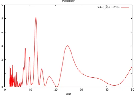
0 1 2 3 4 5 6

0 10 20 30 40 50 year

Periodicity

3-A-2 (1611-1726)

Fig. 8. The same as Fig. 7, but the result is obtained for the

differ-ent sample 3-A-2. Again two clear peaks can be recognized at the periodicities of 12 year and 25 year. The vertical axis represents the power of Fourier analysis.

correspond to the lowest time of O18involved in the tree ring (26.5 per mill).

Furthermore, when we compare present data with the data of Northern Hemisphere temperature anomaly, a good corre-lation has been also found in the time; the high growth rate of the tree ring was observed in the low temperature time of the northern Hemisphere (−0.4◦C) (Mann et al., 1999).

In order to investigate the correlation with the intensity of cosmic rays, we have compared the data of tree growth rate with the data of C14 (Miyahara et al., 2004) and Be10 (Berggren et al., 2009). The highest correlation coeffi-cient (r) between the annual growth rate and C14 has been obtained when the data of C14 (Miyahara et al., 2004) was shifted back 7±1 years. The result turns out asr=0.23 for the number of sampling pointsn=108 with the rejection rate ofP=0.008.

0 1 2 3 4 5 6

0 10 20 30 40 50 year

Periodicity

3-A-3 (1611-1726)

Fig. 9. The same as Fig. 7, but the result is obtained for the different

sample toward the north direction (3-A-3). Again two clear peaks can be recognized at the periodicities of the 12 year and the 25 year. But a 38 year bump appears. This is a ghost peak inherent to 1/3 of the total duration of 115 years. The vertical axis corresponds to the power of Fourier analysis.

0 2 4 6 8 10 12 14

0 10 20 30 40 50

year Periodicity

1-B-2 (1727-1998)

Fig. 10. The result of the analysis to the data set after the Maunder

minimum (1727 and 1998). In comparison with the result presented in Fig. 7, a weak 12 year periodicity is recognized. The analysis is made for the sample 1-B-2. The vertical axis represents the power of Fourier analysis.

On the other hand, in the ice core data of the NGRIP, the excesses of Be10were seen around the years of 1620, 1641, 1674, 1696, 1712, 1715 and 1725 (Berggren et al., 2009). It is surprising to know that except a peak of 1696, the 6 high growth times of present tree ring coincide well with these peaks as shown in Fig. 6. The highest correlation coefficient between the two parameters (r), the annual growth rate of the tree ring and the abundance of Be10, has been obtained when the calendar year of Be10was put back 4±2 years. The correlation coefficient (r) has turned out asr=0.31 with the rejection rate ofP=0.0002 for the sampling pointsn=125. We find out similar discovery by Dengel et al. (2009)

dur-ing the Maunder minimum when the anthropological effect to

(5)

between growth of the trees and the flux density of galactic cosmic radiation in modern times (n=45, r=0.39, P=

0.008). It is worthwhile to mention here that the best corre-lation coefficient was obtained between the two data of Be10 and C14 (Miyahara et al., 2004) when the calendar year of C14 was put back 6±2 years. The r was 0.37 forn=105 withP=0.00005.

3.3 Results of analysis by Lomb method and

Wavelet method

Now we describe the results of the search for the periodicity. At first we have tested our data by a simple Fourier analysis (Press et al., 1992, Lomb method) and searched the existence of any periodicity in the sample. Although the method pro-duces sometimes ghost periodicities that arise from the to-tal duration of the sample, we can find out any periodicity naively if they exist.

When we apply this method to the integral data (annual growth area) between 1611 and 1726, we have found two peaks at 12 years and 25 years as shown in Fig. 7 for the di-rection of 1-B-2 of the wood piece #1. However when we apply the Lomb method (Fourier analysis) to the total data set during 1606 and 1998, we could not find out any clear signals which may link with the solar activity.

To make present discovery sure, we have made the same analysis to the other piece of the wood ring (#3). For the west direction (3-A-2), as shown in Fig. 8, again a clear 12 year peak and a 25 year peak have been seen. For the north di-rection (3-A-3), still a 12 year peak and a 25 year peak can be seen as shown in Fig. 9. However a 38 year ghost peak has appeared. On the other hand for the south direction (1-B-3), the 12 year peak and the 25 year peak have been still clearly recognized, but another 18 year peak was amplified as the same level of the 12 year peak. When we apply the same method to the remaining data between 1727 and 1998, only a weak 12 year peak has been recognized (Fig. 10).

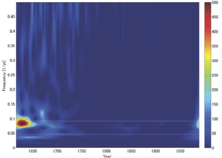
Since the Lomb method does not specify the duration when the periodicity appears strongly and also restricted by the total length of duration, we have analyzed the differential data (width) by the Wavelet analysis (Torrence, 1998; Chui, 1992) . We took the 20 year running average of the growth rate and considered deviations from these averages as the an-nual growth rate. In the time of the data analysis we removed 10 years from each end of the data set and applied the wavelet analysis between the years 1617 and 1988.

Quite surprisingly, we also found an 11 year periodicity in the growth rate during the Maunder minimum, but no strong correlation with 11 years was found after the Maunder min-imum. The result by the wavelet analysis is consistent with previous results obtained by the Lomb method. The results are shown in Fig. 11. The red color corresponds to an ex-cess (an increase in the growth rate) with a very high statis-tical significance. From Fig. 11, there is also some evidence of a weak 25 year periodicity during the Maunder minimum

Fig. 11. Wavelet analysis performed to the annual width data

(dif-ferential data) of 20 year running average. We removed 10 years from both sides and the analysis was performed to the data dur-ing 1617 and 1988. An 11 year periodicity can be seen durdur-ing the Maunder minimum and some evidence is observed for a 25 year pe-riodicity during the Maunder minimum. The red color corresponds to an excess with a very high statistical significance. This has been confirmed by the Monte Carlo simulation.

with a moderate statistical significance. We conclude that our analysis on the annual growth rate clearly shows a possible effect of solar activity to the climate. However we could not confirm the prediction given by Dengel et al. in recent days.

4 Discussions

4.1 Effect of solar irradiance to the Earth

Recently Lean and Rind have analyzed plenty of climate data of the world from 1889 to 2006. They have selected four parameters and estimated each effect to the climate (Lean and Rind, 2008). According to their analysis;

(1) The effect of El-Nino Southern Oscillation (ENSO) im-pacts the zone of 25◦N and 25◦S of the latitude be-tween the equator. The change of the temperature was estimated as to be 1.0 K at the maximum. As well known the peak was observed over the west coast of South America.

(2) The effect of the volcanic ashes and aerosols was widely observed in the region between 70◦N and 40◦S of the latitude. The effect was estimated as to be−0.25 K. The amount of the effect to the climate was estimated by being based on the Pinatubo eruption from November 1991 to September 1992.

(6)

(4) Most interesting effect related with current topics is the effect of solar irradiance on the global climate. Accord-ing to the analysis by Lean and Rind, the global effect was estimated as to be 0.17±0.01 K between the so-lar maximum and minimum. They noticed that the ef-fect appeared strongly in the zone; between 70◦N and 30◦N and between 25◦S and 50◦S of the latitude. The effect works for positive direction and at the peak lati-tude (near 40◦) it was estimated as to be+0.5 K. Later we will discuss being based on this number.

4.2 Effect of solar activity to the width of tree ring

Here we shall discuss why the solar activity has been recorded in the tree ring. It would be natural to think that the growth rate was affected by the local climate and the local climate was influenced by the solar activity (Lean and Rind, 2008). It might arise from the reason that the formation of mist, fog and rain was also modulated by solar activity. For the growth of trees, the abundance of the water is very impor-tant. Even the trees absorb the water vapor from the stomata and grow. Therefore solar activity is registered in the tree rings (Tanaka, 2010).

Now we must reply to the question why Dengel et al. found the 11 year periodicity in the recent tree rings and why we did not observe such a periodicity in our old tree at the same time (1953-1998). One of the possibilities arises from a difference of the growth rate of the tree ring itself. In the young time the annual growth rate of the tree ring is wide, while in the old time the width becomes narrower. Present sample of the tree ring shows quite narrow growth rate in the outer region, so that we could not find out a clear signal of solar activity in the outer region of the tree ring. Just it may arise from a difference inherent to the sample itself.

4.3 A possible mechanism of transportation of solar

activity to tree ring

Here we shall discuss on a possible transportation mecha-nism of solar activity to the growth rate of the tree. The Sun emits in all region of the electromagnetic spectrum; 41% of the energy is emitted in the visible region, 52% is in the in-frared region and 7% in the near ultra-violet region. The en-ergy emitted in the region ofX−ray and ultra-violet ranges constitutes only 0.001% of the total energy emitted (Audouz and Israel, 1996). By the measurement of the NIMBUS 7 satellite, the irradiance changed as±0.1% by the solar activ-ity (Hoyst and Schatten, 1993; Hoyst et al., 1992).

The data ofδC13 indicates that the local temperature of Japan in the Maunder minimum was estimated as to be 3◦cooler than the average (Kitagawa and Matsumoto, 1995). The effect of the solar variation between the solar maximum and minimum to the local climate at the zone of 40◦during these 120 years has been estimated by Lean and Rind as to be 0.5 K (Lean and Rind, 2008). Therefore we can say that

the solar irradiance during the Maunder minimum must be 6 times cooler than the normal time of the solar activity.

Nowadays it is well accepted that the change of 1 Watt/m2 Total Solar Irradiance (TSI) induces the change of the global temperature as 0.1 K (Kamide and Lean , 2008). At the zone of 40◦_{N and S, the difference is enhanced as up to 0.5 K}

be-tween the solar maximum and the minimum. If the global temperature would be reduced by 0.6 K during the Maunder minimum, the temperature of the 40◦N and S must be re-duced as 3◦. Therefore if TSI would be reduced 6 Watt s/m2, the cool temperature of the Maunder minimum would be re-alized. In other words, the reduction of the local temperature of 0.5 K was induced by the variation of TSI from 1374 to 1371.5 Watt s/m2. In order to realize 3◦decrease of the lo-cal temperature, if the Solar constant varied from 1374 to 1368 Watt s/m2, it would be realized. Therefore we estimate that the change of the TSI in the Maunder minimum must be 0.44 percent while the change of the TSI during recent 120 years was about 0.20% (Haigh, 2003; Lean et al., 1995). The decrease of the TSI must be realized in the region of the short wave length of the light; near ultra-violet region, not in the optical and infra-red regions. This may be a reason why our tree ring recorded the past variation of climate change during the Maunder minimum.

4.4 Annual growth rate of trees

(7)

5 Conclusions

We analyzed the annual growth rate of a cedar tree that had survived in Japan for 391 years. We found an 12 year period-icity in the growth rate during the Maunder minimum, but no strong correlation with 12 years was found after the Maunder minimum. The result by the wavelet analysis is consistent with the results obtained by the Lomb method.

A good correlation between our data (annual growth rate of the tree rings) and the Northern Hemisphere mean temper-ature anomaly data during the Maunder minimum is found (Yamguchi et al., 2010). Our data also shows good correla-tions with the peaks of Be10 and C14(Berggren et al., 2009; Miyahara et al., 2007). Therefore it would be natural to think that the growth rate was affected by the local climate and the local climate was influenced by the solar activity (Lean and Rind, 2008). It is interesting to know that even the sun spot disappeared from the solar surface, the dynamo clock worked regularly during the Maunder minimum. Once again we de-scribe our conclusion here that our analysis on the annual growth rate clearly shows a possible effect of solar activity to the climate.

Acknowledgements. The authors acknowledge Prof. O. Tanaka,

Department of Biology of Konan University for valuable discus-sions. They also thank Dr. T. Mitsutani of Nara National Research Institute for Culture Properties for very valuable comments from a point of view of the dendorochronology.

Edited by: H. Fichtner

Reviewed by: A. Mangini and two other anonymous referees

References

Arslanov, Kh.: Radio-Carbon, publ. Geographic Res. Inst., St. Pe-tersburg State University, 1987 (in Russian).

Audouz, J. and Israel, G.: Cambridge Atlas of Astronomy, 19, 1996. Berggren, A. M., Beer, J., Possnert, G., Aldahan, A., Kubik, P., Christl, M., Johnson, S. J., Abreu, J., and Vinther, B. M.: A 600-year annual Be10record from the NGRIP ice core, Greenland, Geophys. Res. Lett., 36, L11801, doi:10.1029/2009GL038004, 2009.

Chui, C. K.: An introduction to wavelet analysis, Acad. Press, 1992. Dengel, S., Aeby, D., and Grace, J.: A relationship between galactic cosmic radiation and tree rings, New Phytologist, 184, 545–551, doi:10.1111/j.1469-8137, 2009.

Eddy, J.: The Maunder Minimum, Science 192, 1189–1202, doi:10.1126/science.192.4245.1189, 1976.

Haigh, J. D.: The effect of solar variability on the Earths climate, Phil. Trans. R. Soc. Lond., A361, 95–111, 2003.

Hoyst, D. and Schatten, K. H.: A discussion of plausible solar irra-diance variation, J. Geophys. Res., 98, 18895–18906, 1993. Hoyst, D. V., Lee kyle, H., Hickey, J. R., and Maschhoff, R. H.:

The Nimbus 7 Solar Total Irradiance: a new algorithm for its deviation, J. Geophys. Res., 97, 51–63, doi:10.1029/9/JA02488, 1992.

Kamide, K. and Lean, J. J.: Solar Constant and Global Climate, in: Proc. 5th Space Craft Environment Symposium at JAXA sympo-sium, JAXA-SP-08-018, ISSN 1349-113X, 2008.

Kitagawa, H. and Matsumoto, E.: Climate implication ofδC13 vari-ation in Japanese cedar (Cryptomeria japonica) during the last two millenniums, Geophys. Res. Lett., 22, 2155–2158, 1995. Kocharov, G. E., Ostryakov, G. E., Peristykh, A. N., Vasilev, V. A.:

Radiocarbon content variation and Maunder Minimum of Solar Activity, Solar Phys., 181, 381–391, 1995.

Kononov, Yu. M., Friedrich, M., and Boettger, T.: Regional Sum-mer Temperature Reconstruction in the Khibiny Low Mountain (Kola Peninsula, NW Russia) by means of Tree-ring Width dur-ing the Last Four Centuries, Arctic, Antarctic and Alpine Res., 41, 460–468, doi:10.1657/1938-4246-41.4.460, 2009.

Kulmala, M., Hari, P., Riipinen, I., and Kerminen, V-M.: On the possible links between tree growth and galactic cosmic rays, New Phytologist, 184, 511–513, doi:10.1111/j.1469-813, 2009. Lean, J. L. and Rind, D. H.: How natural and

anthro-pogenic influences alter global and regional surface tempera-tures: 1889 to 2006, Geophys. Res. Lett., 35, L18701, doi. 10.1029/2008GL034864, 2008.

Lean, J., Beer, J., and Bradley, R.,: Reconstruction of solar irradi-ance since 1610: implication for climate change, Geophys. Res. Lett., 22, 3195–3198, 1995.

Mann, M. E., Bradley, R. S., and Hughes, M. K.: Northern Hemi-sphere Temperature during the Past Millennium: Influences, Un-certainties, and Limitations, Geophys. Res. Lett., 26, 759–762, 1999.

Mitsutani, T.: private communication, 2011.

Miyahara, H., Masuda, K., Muraki, Y., Furuzawa, H., Menjo, H., and Nakamura, T.: Cyclicity of solar activity during the Maunder Minimum deduced from radiocarbon content, Solar Phys., 224, 317–322, 2004.

Miyahara, H., Masuda, K., Nagaya, K., Kuwana, K., Muraki, Y., and Nakamura, T.: Variation of solar activity from the Spoerer to the Maunder minima indicated by the radiocarbon content in tree rings, Adv. Space Res., 40, 1060–1063, 2007.

Press, W. H., Teukolsky, S. A., Vetterling, W. T., and Flannery, B. P.: Numerical Recipes,in C, Cambridge Univ. press, 575, 1992. Solanki, S. K. and Fligge, M.: Solar Irradiance since 1874

Revis-ited, Geophys. Res. Lett., 25, 341–344, 1998.

Stueiver, M., Reiner, P. J., and Braziunas, T. F.: High-precision ra-diocarbon age calibration for terrestrial and marine samples, Ra-diocarbon, 40, 1127–1151, 1998.

Svensmark, H.: Influence of Cosmic rays on Earths Climate, Phys. Rev. Lett., 81, 5027–5030, 1998.

Svensmark, H.: Cosmoclimatology, Astron. Geophys., 48, 1.18– 1.21, 2007.

Svensmark, H. and Friis-Christensen, E.: Variation of cosmic ray flux and global cloud coverage- a missing link in solar-climate relationships, J. Atmos. Sol. Terr. Phys., 59, 1225–1232, 1997; Tanaka, O.: private communication (2010).

Torrence, C. and Campo, G. P.: A practical guide to Wavelet analy-sis, Bull. Am. Meteorol. Soc., 79, 61–78, 1998.