Robust Statistical Pearson Correlation Diagnostics for Bitcoin Exchange Rate with Trading Volume: An Analysis of High Frequency Data in High Volatility Environment

(1)

https://dx.doi.org/10.24001/ijaems.3.12.7 ISSN: 2454-1311

Robust Statistical Pearson Correlation

Diagnostics for Bitcoin Exchange Rate with

Trading Volume: An Analysis of High Frequency

Data in High Volatility Environment

Nashirah Abu Bakar

1

_{, Sofian Rosbi}

2

1_{Islamic Business School, College of Business, Universiti Utara Malaysia, Malaysia}

2_{School of Mechatronic Engineering, Universiti Malaysia Perlis, Malaysia}

Abstract—Crptocurrency is a digital or virtual currency that uses cryptography for security, transfer process and storage in ledger. This paper is to validate the correlation between exchange rate changes and trading volume changes. Data selected for this study is hourly data starting from 4 November 2017 until 7 November 2017. Methodology implemented in this study started with normality diagnostics and followed by correlation diagnostic. In this study, Pearson correlation calculation is implemented to evaluate the association between two variables namely exchange rate and trading volume. Pearson's correlation coefficient (r) is a measure of the strength of the association between the two variables. Result shows the coefficient of association is 0.123. Therefore, this study proved that the association between exchange rate changes and trading volume changes is very weak association. This value occurred because there is high volatility in hourly data and existence of outliers. The significant of this finding will help investors to recognize the relationship between trading volume and exchange rate. Therefore, it will help investors to make better decision in developing investment portfolio.

Keywords— Bitcoin, Volatility, Correlation, Exchange rate, Trading volume.

I. INTRODUCTION

Bitcoin cryptocurrency is defined as a digital currency in which encryption techniques are used to regulate the generation of units of currency. Bitcoin cryptocurrency involve with a complex process with the bitcoin cryptocurrency in which encryption techniques are used to regulate the generation of units of currency. Then the system will verify the transfer of funds, operating independently from central bank. It is, however, not subject to regulation by central banks, does not enjoy the backing of goods or services with intrinsic value (Rees, 2014).

Abu Bakar et al. (2017) explains the process of bitcoin cryptocurrency transaction procedure was started with the User A transfer digital currency to User B. The transaction needs to go through the blockchain path. A

blockchain is an open, distributed ledger that

can record transactions between two parties efficiently and in a verifiable and permanent way (Reid and Harrigan, 2013). A transaction is a transfer of bitcoin value that is broadcast to the network and collected into blocks. A transaction typically references previous transaction outputs as new transaction inputs and dedicates all input bitcoin values to new outputs (Miers, et al., 2013). Ledger is open to all users in the networks, and all users refer to one public ledger of transaction chain (Moore and Christin, 2013).

Cryptocurrency make it easier to transfer funds between two parties in a transaction; these transfers are facilitated using public and private keys for security purposes. These fund transfers are done with minimal processing fees, allowing users to avoid the steep fees charged by most banks and financial institutions for wire transfers. Cryptocurrency defines an electronic coin as a chain of digital signatures (Okamoto, 1995). Each owner transfers the coin to the next by digitally signing a hash of the previous transaction and the public key of the next owner and adding these to the end of the coin. A payee can verify the signatures to verify the chain of ownership. Bitcoin miners help keep the Bitcoin network secure by approving transactions (Kroll et al., 2013). Mining is an important and integral part of Bitcoin that ensures fairness while keeping the Bitcoin network stable, safe and secure (Ron and Shamir, 2013).

(2)

between exchange rate changes and trading volume changes.

II. LITERATUREREVIEW

Bitcoin cryptocurrency is difference from conventional currency because it is not a fiat money or specific money. Bitcoin also not regarded as legal tender by a central authority or backed by goods or services having an intrinsic value (Christopher, 2014) and bitcoin is also decentralised in the sense that it is not issued by a government or single institution (Ram, et al, 2016). The price of bitcoin is based on supply and demand. The exchange rate of cryptocurrency fluctuate widely depend on news or speculations (Abu Bakar and Rosbi, 2017). According to Abu Bakar and Rosbi (2017), bitcoin cryptocurrency involved with high volatility. They found the standard error for Bitcoin volatility is 4.458 % show as high value of volatility.

A defining feature of a cryptocurrency and arguably its most endearing allure is its organic nature; it is not issued by any central authority, rendering it theoretically immune to government interference or manipulation (Bohme, et al., 2015). Most cryptocurrencies are designed to gradually decrease the production of currency, placing an ultimate cap on the total amount of currency that will ever be in circulation, mimicking precious metals (Barber, et al., 2012).

Abu Bakar and Rosbi (2017) conclude that a bitcoin transaction is a transfer of bitcoin value that is broadcast to the network and collected into blocks. A transaction typically references previous transaction outputs as new transaction inputs and dedicates all input bitcoin values to new outputs. Transactions are not encrypted, so it is possible to browse and view every transaction ever collected into a block. Once transactions are buried under

enough confirmations, they can be considered

irreversible. This system is vulnerable to hacking activity. Bitcoin cryptocurrency also has no physical form and exists only in a network. Bitcoin cryptocurrency is no intrinsic value in that it is not redeemable for another commodity, namely gold.

III. RESEARCHMETHODOLOGY

This section describes the methodology implemented in

this study starting from data selection, data

transformation, normality diagnostics and Pearson correlation diagnostics. This study performed Pearson correlation analysis for exchange rate changes to trading volume changes.

3.1 Data selection

There are two variables are selected in this study namely exchange rate (USD/Bitcoin) and total trading volume

from 4 November 2017 until 7 November 2017.These

data are collected from https://www.worldcoinindex.com.

3.2 Mathematical derivation for exchange rate

changes and trading volume changes

This study evaluates the correlation between exchange rate changes and trading volume changes. Therefore, calculation for exchange rate and trading volume changes need to be derived.

Firstly, this study derived the percentage changes for exchange rate using Equation (1).

1 1

100 %

t t t

EX EX

EX

 

  

 _ _

  ………...……. (1)

Where:

EX

 is percentage changes of exchange rate,

t

EX is exchange rate value for trading period t and

1

t

EX_ is exchange rate value for trading period t-1.

Next, this study derived the percentage of changes for trading volume as stated in Equation (2).

1 1

100 %

t t t

TV TV

TV

 

  

 _ _

  ……… (2)

where:

TV

 is percentage changes of exchange rate,

t

TV is exchange rate value for trading period t and

1

t

TV is exchange rate value for trading period t-1.

3.3 Normality statistical test

The probability density of the normal distribution is:

 

2 2

1

2

x

f x e

 



 

 ……… (3)

Where:



is the mean or expectation of the distribution,

 is standard deviation, and

2

 is variance for data distribution.

Properties of a normal distribution:

(a) The mean, mode and median are all equal. (b) The curve is symmetric at the center. Data are

distributed around the mean, μ.

(c) Exactly half of the values are to the left of center and exactly half the values are to the right. (d) The total area under the curve is 1.

(3)

The Shapiro-Wilk test is a method to evaluate whether a random sample comes from a normal distribution. The test gives you a W value. The W value larger than chosen alpha (0.05), will concludes the distribution of data follows normal distribution. The, if the data shows small values of W, it is indicate your sample is not normally distributed. The formula for the W value is:





2

( ) 1

2

1

n

i i

i n

i i

a x

W

x





















where:

i

xis the value in the sample



x x x₁, ₂, ₃,...,xn



;

( )i

x is the ordered sample values ,(x₍₁₎is the smallest

value in the sample);



x1 x2 .... xn



x

n

  

 is the sample mean;

i

a is constants that derived generated from the means,

variances and covariances of the order statistics of a

sample of size n from a normal distribution. The

calculation of a_iis described in below equation.









T 1

1 2 3 1/ 2

T 1 1

, , ,..., _n m V

a a a a

m V V m

  



where:

V

is the covariance matrix of those order statistics;





T

1, 2, 3,..., n

m m m m m

Element in Equation (8) is represented as:

1, 2, 3,..., n

m m m m are the expected values of the order

statistics of independent and identically distributed random variables sampled from the standard normal distribution

3.4 Pearson correlation diagnostics

The Pearson product-moment correlation coefficientis a measure of the strength of a linear association between

two variables and is denoted by r. The Pearson

product-moment correlation develops a line of best fit through the data of two variables. Then, the Pearson correlation

coefficient, r, indicates how well the data points fit this

modeling line.

Consider the Pearson product-moment correlation

coefficient of two n-dimensional vectors X ={X1,

X2,...,Xn} and Y = {Y1,Y2,...,Yn}. Pearson correlation is

states as the ratio between the covariance of X and Y and

the product of their standard deviations. Pearson's correlation coefficient when applied to a population is commonly represented by below equation:





,

cov ,

X Y

X Y

X Y



 



where cov is the covariance, _X is the standard

deviation of X, and _Y is the standard deviation of Y.

Then, covariance expressed as below:







cov( , )X Y E_ X



_X Y



_Y _

where E is the expectation and _X is the mean of X.

Therefore, Equation (12) can be written as:







,

X Y

X Y

X Y

E X  Y 



 

 

 

 



Then, mathematical equation for ρ can be expressed in

terms of uncentered moments. Mean of population is expressed as next equation,

 

E

X X



 ,



_Y E

 

Y

Variance of population is expressed as next equation,

 





 



 



   



 



 



 



 

2 2

2

2 2

E E E 2 E

E 2E E E

E 2E E

E E

X X X X X X E X

X X X X

X X X

X X

  _  _ _   _

 

 _ _ 

 

 _ _ 

 

 _ _

 

2

2 2

E E

Y Y Y



  _{ }

Standard deviation of population is expressed as next equation,

 

2

E E

X X X

  _ _ ,

 

2 2

E E

Y Y Y

   _{ }

Covariance of population is expressed as next equation,







 







 



 

     





             

     

E

E E E

E E E E E

E E E E E E E

E E E

X Y

X X Y Y

XY X Y Y X X Y XY X Y X Y X Y XY X Y

 

 

 

 

 

 _   _

 

 _    _

   

 

Therefore, Equation (14) can be represented as:

     

 

, ₂ ₂

2 2

X Y

E XY E X E Y

E X E X E Y E Y

  

 _ _  _ _

   

Then, the equation for sample is derived. Sample Pearson's correlation coefficient is commonly represented by the letter r. Consider the sample of dataset x =

{x1,...,xn} containing n values and another dataset y =

{y1,...,yn} containing n values then that formula for r is:

,

cov( , )

x y

x y

x y r

(4)

where cov is the covariance,

s

_x is the standard deviation

of x, and

s

_y is the standard deviation of y.

Then, sample covariance can be expressed as below:

 

1







sample cov ,

1

n

i i

i

x x y y

x y n     



Therefore, Equation (16) can be written as:

Then, mathematical equation for r can be expressed in

terms of uncentered moments. Mean of sample,

1 n i i x x n  



, 1 n i i y y n  



Variance of sample,









 





 

2

2 2 2

1 1 2 1 2 2 ₁ 1 2 2 1 1 2 2 1 1 1 1

[ ] 2

1 1 1 1 1 1 1 1 1 1 n n

x i i i

i i n i i n i n i i i n i n i i i n n i i i i

s x x x x x x

n n

x nx x n x x n n n x x n n

n x x n n                    _  _     _ _   _ _   _ _   _  _     _ _       _ _   _ _       _  _         _ _    _ _   _   _











 

2 2 1 2 2 1 1 1 1 1 1 n y i i n n i i i i

s y y n

n y y n n        _ _    _ _   _   _



Standard deviation of sample,





 

2 2 1 1 1 1 n n

x i i

i i

s n x x

n n  

 _ _    _ _   __



_



_ __





 

2 2 1 1 1 1 n n

y i i

i i

s n y y

n n  

 _ _ 

  _ _ 

 __



_



_ __

Covariance of sample,

 











1

1 1 1 1

1 1 1 1 cov , 1 1 1 1 1 1 1 1 2 1 1 1 1 1 n i i i n

i i i i i

n n n n

i i i i

n i i i n i i i n i i i n i i i i x y

x x y y n

x y x y xy x y n

x y x y y x x y n

x y nx y ny x nx y n

x y nx y nx y n

x y nx y n

x x y n

n n                       _    _       _    _       _   _       _  _        







1 1 1 1 1

1 1 1

1 1 1 1 n i n i i n i n n i i i i

i i

n n n

i i i i

i i i

y n

y x y x

n n

n x y x y n n                            _ _                     _ _      _  _   



 

Therefore, Equation (18) can be represented as:

 

1 1 1

,

2 2

1 1 1 1

n n n

i i i i

i i i

x y

n n n n

i i i i

n x y x y

r

n x x n y y

                _ _   _ _     _ _   _ _             



 



IV. RESULTANDDISCUSSIONS

This section describes the result for statistical test of normality data characteristics. Then, this study performs Pearson correlation diagnostics to evaluate the association between changes of exchange rate with changes of trading volume.

(5)

03:00. Meanwhile, the minimum value is 6,996.70 USD on 7 November 2017, 16:00.

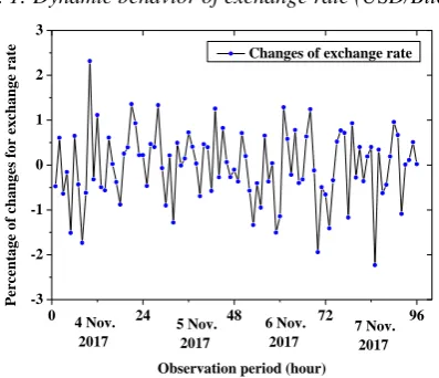
Then, this study calculated the percentages of changes with respect to previous observation period. Figure 2 shows percentage of changes for exchange rate of Bitcoin.

0 24 48 72 96 6900

7000 7100 7200 7300 7400 7500 7600 7700

7 Nov. 2017 6 Nov.

2017 5 Nov. 2017

E

x

ch

a

n

g

e r

a

te

(

U

S

D

/

B

it

co

in

)

Observation period (hour)

Exchange rate

4 Nov. 2017

Fig. 1: Dynamic behavior of exchange rate (USD/Bitcoin)

0 24 48 72 96 -3

-2 -1 0 1 2 3

7 Nov. 2017 6 Nov.

2017 5 Nov.

2017

Pe

r

c

e

n

tage

of

c

h

an

ge

s for

e

xc

h

an

ge

r

at

e

Changes of exchange rate

4 Nov. 2017

Fig. 2: Percentage of changes for exchange rate

The maximum value is 2.3168 on 4 November 2017, 10:00. Mean of the data distribution is -0.0301 and standard deviation is 0.79764.

Next, this study validates the normality characteristics finding using histogram, normal probability plot and statistical test. Figure 3 shows the histogram of exchange rate changes. The distribution of exchange rate changes follows the normal distribution line. Figure 4 is normal probability plot of exchange rate changes in percentages. Data distribution is near to normal distribution line. Therefore, the data distribution is follow normal distribution.

Then, this study validated the normality using Shapiro-Wilk normality test. Table 1 shows the Shapiro-Shapiro-Wilk normality statistical test. The p-value is 0.567. Therefore, the data distribution is follow normal distribution.

-2 -1 0 1 2

0 5 10 15 20 25 30

F

re

qu

ency

Changes of exchange rate (%) Exchange rate changes

Fig. 3: Histogram of exchange rate changes

-3 -2 -1 0 1 2 3 0.01

1 10 40 70 95 99.5

Normal Probability Plot of Exchange Rate Changes (%) mean = -0.0301 standard deviation = 0.79764

Nor

m

al Pe

rc

en

til

es

Changes of exchange rate (%)

Percentiles Reference Line

Fig. 4: Normal probability plot of exchange rate changes Table 1: Normality test using Shapiro-Wilk

Shapiro-Wilk test

Statistics Degree of

freedom

Probability value Exchange

rate changes 0.988 96 0.567

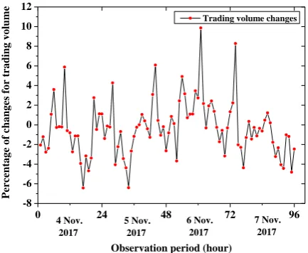
3.2 Normality characteristics of trading volume data This section describes the normality checking for trading volume data. Data selected in this study involving data of trading volume starting from 4 November 2017, 0:00 until 7 November 2017, 24:00. The minimum value of

trading volume is 1.860x109_{USD on 5 November 2017,}

18:00. Meanwhile, the maximum value of trading volume

is 2.998 x109_{USD on 4 November 2017, 10:00.}

(6)

0 24 48 72 96 1.6x109

1.8x109

2.0x109 2.2x109 2.4x109 2.6x109 2.8x109

3.0x109 3.2x109

7 Nov. 2017 6 Nov.

2017 5 Nov.

2017

Trading volume (USD)

Observation period (hour) Trading volume (USD)

4 Nov. 2017

Fig. 5: Dynamic behavior of total trading volume (USD)

0 24 48 72 96

-8 -6 -4 -2 0 2 4 6 8 10 12

7 Nov. 2017 6 Nov.

2017 5 Nov.

2017

Pe

rc

en

tage

of

c

h

an

ge

s for

t

rad

in

g volu

m

e

Trading volume changes

4 Nov. 2017

Fig. 6: Percentage of changes in trading volume

Next, this study performed normality test diagnostics to evaluate the data distribution of changes for trading volume data. This study implemented graphical approach and numerical statistical test approach to validate the normality of data distribution.

Figure 7 shows the histogram for trading volume changes in percentage. The distribution is near to normal line. However, there are outliers in right side of normal distribution. Figure 8 shows the normal percentiles plot for trading volume changes. The distribution of data is near to reference line. Figure 8 indicates the present of outliers.

Table 2 shows the numerical prove of normality statistical test using Shapiro-Wilk approach. Probability value is 0.004. Therefore, data distribution is deviate from normal distribution. The presence of the outliers contributes to the non-normal distribution of data.

-12 -10 -8 -6 -4 -2 0 2 4 6 8 10 12 0

5 10 15 20 25 30 35 40

Fr

equency

Changes of trading volume (%)

Changes of trading volume

Fig. 7: Histogram of trading volume changes

-10 -5 0 5 10

0.01 1 10 40 70 95 99.5

Normal Probability Plot of Trading Volume Changes (%) mean = -0.38392 standard deviation = 2.82637

Normal Percentiles

Trading volume changes (%)

Percentiles Reference Line

Fig. 8: Normal percentiles for trading volume changes Table 2: Normality test using Shapiro-Wilk

Shapiro-Wilk test

Statistics Degree of

freedom

Probability value Trading

volume changes

0.959 96 0.004

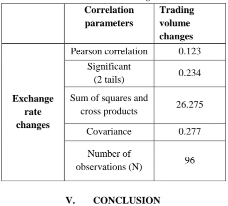
3.3 Correlation diagnostics of exchange rate changes with trading volume changes

This section describes the correlation analysis between exchange rate changes with trading volume changes. Analysis that implemented in this section is using Pearson correlation method.

First, this study validated the correlation using graphical method namely scatter plot between two variables. Figure 9 shows the scatterplot graph between trading volume changes and exchange rate changes.

(7)

-10 -8 -6 -4 -2 0 2 4 6 8 10 12

-3 -2 -1 0 1 2 3

E

x

ch

a

n

g

e r

a

te

c

h

a

n

g

es

(

%)

Trading volume changes (%)

Fig. 9: Normal percentiles for trading volume changes Table 2: Correlation diagnostics

Correlation parameters

Trading volume changes

Exchange rate changes

Pearson correlation 0.123

Significant

(2 tails) 0.234

Sum of squares and

cross products 26.275

Covariance 0.277

Number of

observations (N) 96

V. CONCLUSION

This objective of this study is to develop robust Pearson correlation diagnostics between trading volume changes and exchange rate changes. Data selected in this study are collected hourly starting from 4 November 2017, 0:00 until 7 November 2017, 24:00.Main findings of this study are described as below.

(a) In this study , two variables of data is collected

namely exchange rate (USD/Bitcoin) and total trading volume (USD).Both of the variables are collected in hourly starting from 4 November 2017, 0:00 until 7 November, 24:00.

(b) This study calculated the percentages of exchange

rate changes with respect to previous observation period. The maximum value is 2.3168 on 4 November 2017, 10:00. Mean of the data distribution is -0.0301 and standard deviation is 0.79764.

(c) This study validated the normality of exchange rate

changes using Wilk normality test. Shapiro-Wilk normality statistical test shows the p-value is 0.567. Therefore, the data distribution is follow normal distribution.

(d) Then, this study calculated the percentage of changes

in the trading volume. The analysis shows the mean of the data distribution for changes of trading volume is -0.38392. In addition, the standard deviation of data distribution for trading volume changes is 2.82637.

(e) Next, this study performed the numerical prove of

normality statistical test using Shapiro-Wilk

approach for trading volume changes. Probability value is 0.004. Therefore, data distribution is deviate from normal distribution. The presence of the outliers contributes to the non-normal distribution of data.

(f) Next, this study validates the association between

trading volume changes and exchange rate changes using Pearson correlation analysis. Numerical result shows the Pearson correlation is 0.123 that indicates very weak positive correlation.

The findings of this study are important to investors and economics expert to validate the dynamic behavior of exchange rate associated with trading volume. High volatility environment contributes to the non-normality data distribution. In the same time, high frequency data for Bitcoin also indicates high volatility .Therefore, the finding of this study shows there is very weak positive correlation between trading volume changes and exchange rate changes.

REFERENCES

[1] Abu Bakar, N. and Rosbi, S. (2017), Autoregressive

Integrated Moving Average (ARIMA) Model for Forecasting Cryptocurrency Exchange Rate in High Volatility Environment: A New Insight of Bitcoin

Transaction, International Journal of Advanced

Engineering Research and Science, Vol. 4 (11), pp. 130-137

[2] Abu Bakar, N. and Rosbi, S. (2017), High Volatility

Detection Method Using Statistical Process Control for Cryptocurrency Exchange Rate: A Case Study of

Bitcoin, The International Journal of Engineering

and Science, Vol. 6 (11), pp. 39-48

[3] Abu Bakar, N., Rosbi, S. and Uzaki, K. (2017),

Cryptocurrency Framework Diagnostics from Islamic Finance Perspective: A New Insight of Bitcoin

System Transaction, International Journal of

Management Science and Business Administration, Vol. 4(1), pp. 19-28

[4] Christopher, C.M. (2014), Whack-a-mole: why

prosecuting digital currency exchanges won’t stop

online laundering, Lewis and Clark Law Review, Vol. 1(1).

[5] Rees, M. (2014), Bitcoin to earth: don’t look now,

but your paradigm is shifting”, Bitcoin Magazine,

(8)

http://bitcoinmagazine.com/15054/bitcoin-earth-dont-look-nowparadigm-shifting/ (accessed 9

December 2017).

[6] Ram, A., Maroun, W. and Garnett, R. (2016)

Accounting for the Bitcoin: accountability,

neoliberalism and a correspondence analysis, Meditari Accountancy Research, Vol. 24 Issue: 1, pp.2-35

[7] Reid,F. and Harrigan,M., "An analysis of anonymity

in the Bitcoin system," in Privacy, security, risk and trust (PASSAT), 2011 IEEE Third Internatiojn Conference on Social Computing (SOCIALCOM). IEEE, 2011, pp. 1318-1326.

[8] Miers,I.,Garman, C.,Green,M. and Rubin, A. D.

"Zerocoin: Anonymous Distributed E-Cash from Bitcoin," 2013 IEEE Symposium on Security and Privacy, Berkeley, CA, 2013, pp. 397-411.doi: 10.1109/SP.2013.34

[9] Moore, T., and Christin, N. (2013, April). Beware the

middleman: Empirical analysis of Bitcoin-exchange

risk. International Conference on Financial

Cryptography and Data Security (pp. 25-33). Springer, Berlin, Heidelberg

[10]Okamoto, T.: An Efficient Divisible Electronic Cash

Scheme. In: Coppersmith, D. (ed.) CRYPTO 1995.

LNCS, vol. 963, pp. 438–451. Springer, Heidelberg

(1995)

[11]Kroll, J. A., Davey, I. C., & Felten, E. W. (2013,

June). The economics of Bitcoin mining, or Bitcoin in the presence of adversaries. In Proceedings of WEIS (Vol. 2013)

[12]Ron D., Shamir A. (2013) Quantitative Analysis of

the Full Bitcoin Transaction Graph. In: Sadeghi AR. (eds) Financial Cryptography and Data Security. FC 2013. Lecture Notes in Computer Science, vol 7859. Springer, Berlin, Heidelberg

[13]Böhme, R., Christin, N., Edelman, B., and Moore, T.

(2015). Bitcoin: Economics, technology, and

governance. The Journal of Economic Perspectives, 29(2), 213-238

[14]Barber, S., Boyen, X., Shi, E. and Uzun, E. "Bitter to