* To whom all correspondence should be addressed. Tel.: +989143524238; Fax: +981824322205; E-mail: [email protected]
The Effect of Ordering Policy Based on Extended Time-Delay
Feedback Control on the Chaotic Behavior in Supply Chains
H. Norouzi Nav*1, M.R. Jahed Motlagh2 and A. Makui3
1Department of Electrical Engineering, Science and Research Branch, Islamic Azad University, Tehran, Iran.
2Department of Computer Engineering, Iran University of Science & Technology, Tehran, Iran. 3Department of Industrial Engineering, Iran University of Science & Technology, Tehran, Iran.
doi: http://dx.doi.org/10.13005/bbra/2191
(Received: 15 June 2015; accepted: 24 July 2015)
A supply chain is a complex nonlinear system involving multiple levels and may have a chaotic behavior. The policy of each level in inventory control, demand forecast, and constraints and uncertainties of demand and supply (or production) significantly affects the complexity of its behavior. This paper compares the performance of new ordering policy based on extended time-delay feedback (ETDF) control with the well-known smooth ordering policy on the chaotic behavior in the supply chain. Exponential smoothing (ES) forecast method is used to predict the demand. The effects of inventory adjustment parameter and supply line adjustment parameter on the behavior of the supply chain are investigated. Finally, two scenarios are designed foranalysis the chaotic behavior of the supply chain and in each scenario the maximum Lyapunov exponent is calculated and drawn. Finally, the best scenario for decision-making is obtained.
Key words: Supply chain; Ordering policy; Chaotic behavior; Extended time-delay feedback control.
The chaotic behavior (an unusual behavior of nonlinear dynamics) has been observed in supply chains. Mosekilde and Larsen (1988), Thomsen et al. (1992), Sosnotseva and Mosekilde (1997), and Larsen et al. (1999) have considered a deterministic supply chain and have shown its chaotic behavior. They have classified the behavior of this chain in four groups, namely, stable, periodic, chaotic, and hyperchaotic.
One type of dynamic behavior is caused by marketing and competition activities that create interaction between suppliers and customers. The interaction may generate a chaotic behavior in the supply chain (Jarsulic, 1993; Matsumoto, 2001).The changing of price has a fundamental
effect on customers demand. Usually the demand goes down as price increases and vice versa. Wu and Zhang (2007)showed the chaotic behavior of the supply chain by simulating the interaction between customers and suppliers where customers respond to the price discount offer made by the supplier and the supplier adjusts the price according to stock held.
This paper is concerned with the comparison of the ordering policy based on extended time-delay feedback (ETDF) control (Fradkov and Evans, 2005) to the smooth ordering policy. The particular emphasis of this paper is the impact the two ordering policies have on the chaotic behavior in the supply chain.A general class of multi-level supply chain is provided that has four successive levels based on the beer distribution model. Each level must satisfy demand, control inventory and place an order through interactions with adjacent levels. The exponential smoothing (ES) forecast method is used to forecast demand at all levels.
Two scenarios are designed for examining the chaotic behavior of the supply chain based on the forecast method and two ordering policies. In each scenario, the effects of the inventory adjustment parameter and supply line adjustment parameter on the supply chain behavior are investigated through calculating the maximum LE and then the best scenario is selected.
This paper is organized as follows: Section 2 briefly introduces chaotic systems and the extended time-delay feedback (ETDF) control. The section 3describes a multi-level model of the supply chain and defines its dynamic equations. In addition, the demand forecasting method and ordering policies are assessed. In section 4, a four-level supply chain is simulated with two different scenarios and their results are compared. System Description
Chaotic systems
Chaotic systems are deterministic systems with high complexity and irregular behavior and categorized as nonlinear dynamic systems. There are two common approaches to identify and measure chaos: graphical methods and quantitative methods (Wiggins, 1990; Sprott, 2003). Graphical methods such as time series and phase plots are visible but less accurate, while quantitative methods can determine the degree of chaos.
The Lyapunov exponent (LE) as the most important quantitative method that measures the sensitivity of initial conditions is a standard quantifier for determining and classifying the behavior of nonlinear systems. A wide range of LEs can be theoretically obtained, but the largest LE is of significance importance, which is calculated
as follows(Sprott, 2003):
...(1)
and are the distances between two nearby trajectories at times and , respectively. If all LEs are negative, the system will be stable. In chaotic systems, at least one LE or the largest LE is positive.
Extended time-delay feedback control
During recent years, the method of time-delayed feedback to control a chaotic system has attracted a plenty of research interest (Fradkov and Evans, 2005; Pyragas, 1992). Assume a continuous-time system is described by Eq.(2) as follows:
...(2) where
x
is an -dimensional vector of state variables andu
an -dimensional vector of inputs (control variables).Pyragas (Pyragas, 1992) considered stabilization of a -periodic orbit of the nonlinear system (2) using a simple control low described by Eq.(3) as follows:
...(3)
where is the feedback gain and is a time-delay.
An extended version of the time-delayed feedback method is presented by Eq.(4) as follows (Fradkov and Evans, 2005):
...(4)
where is the
observed output and are tuning
parameters. For , and the
corresponding results for an extended control law (4) were presented in Konishi, Ishii and Kokame (1999) and Nakajima and Ueda (1998).Recently, Pyragas (Pyragas, 2001)suggested using the
controller (5) with . In thismethod, the
controller itselfbecomes unstable while stability of the overall closed-loopsystem can still be preserved.
Model
In this paper, a supply chain with two ordering policies is investigated which, like the beer distribution model, has four successive levels: factory, distributor, wholesaler, and retailer (Fig.1). In this system, orders propagate from customers to factory and products flow from factory to customers.
Each level in the supply chain receives incoming products after a time delay from the time of placing an order. Meanwhile, a new demand is received. Based on their supply capacity, entities fulfill all or part of the backlog and current demand. Operations of each level are represented by Eqs.(6 &7) as follows:
...(6)
...(7)
where is the effective inventory (inventory level after fulfilling the backlog), the
actual supply line (orders placed but not yet received),
) (t oi
the order quantity, di(t)the demand,
and τis a time delaybetween order placement and delivery.
The most importantdecision variablein thesupply chain is the order quantity thathasan essential rolein its behavior. Thispaperexamines two ordering policies. A well-known oneisthe smooth ordering policy whose decision equation isdefined by Eq.(8) as follows:
...(8)
where is the inventoryadjustment parameter and the error between the actual
inventory and the desired inventory :
...(9)
i β
is the supply lineadjustment parameter and ey(t)
i is the error between the actual supply lineyi(t)and the desired supply lineyi(t):
...(10)
) (
ˆ t
di is the demandforecast that is usually
obtained fromexponential smoothing (ES) forecast method:
...(11)
is a parameter whichdetermines how fast expectation are updated.
Aneworderingpolicybased on the ETDF control is used in the model:
...(12) Table1. The initial data and parameters.
Item Value
Initial inventory (in each level) 30 Initial supply line (in each level) 15 Desired inventory (in each level) 20 Desired supply line (in each level) 10
Customer demand, 20
Lead time, 5
Fixed updating parameter for expectations, 0.4 Inventory adjustment parameter, 0 ≤α≤1 Inventory tuning parameter, 0.5α Supply line adjustment parameter , 0≤Α≤1 Supply line tuning parameter, 0.5β
Table 2. The numberof Maximum LEs in different ranges.
Scenario λ max<0 0≤λ max<0.01 0.01≤λ max<00.02 0.02≤λ max
2325 477 543 6655 1
α
i
r and riβ aretuning parameters which are
adjustable. In this policy, thedifference betweentwo successive errors and its past ordersare usedto accelerate decision-making.αiand
i
β
are like thesmoothorderingpolicy.
Simulation
Consider a supply chain with four levels. There are two scenarios for decision-making:smooth ordering policy and ES forecast method (Scenario 1), andordering policy based ETDF control and ES forecast method (Scenario
2). It is assumed that all levels simultaneously use one scenario and their parameters are the same. Initial values and parameters are set according to Table 1. The model is simulated with the MATLAB software and in each scenario, 2000 data points are used to calculate the maximum LE.
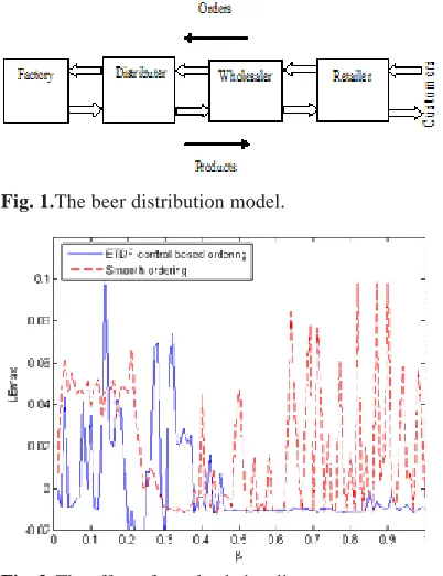
Now with two scenarios, effects of inventory adjustment parameterand supply lineadjustment parameteron the behavior of the supply chain are investigated. Assume that an ES forecast method is used in all levels and the supply lineadjustment parameter is constant at0.1. Change
the inventory adjustment parameter from 0 to 1and
use two ordering policies. The chaotic behavior of the supply chain is studiedthrough calculating the maximum LE. The results show that the ordering policy based on ETDF control(Scenario 2) is suitable, thus the behavior of the supply chain is stable in a greater range of α(Fig. 2). Now, the inventory adjustment parameter is kept constant Fig. 1.The beer distribution model.
Fig. 2. The effect of inventory adjustment parameter.
Fig. 3. The effect of supply chain adjustment parameter.
Fig. 5. Comparison of all scenarios with 01
. 0 0≤λmax ≺
.
( ) and
β
is changed from
0 to 1 to study the effect of the supply lineadjustment parameteron the supply chain (Fig. 3). The maximum LE of both ordering policies is positive in a large range, but with Scenario 2, the chaotic behavior of supply chain is less intense (Fig. 3). In addition, the stability range is larger with this scenario.
For greater certainty, maximum LE is recalculated by changing α and with an increment of
01 . 0
from 0to 1 in two scenarios.
The numberof Maximum LEs in different ranges is showninTable2. In the stablestate ( ),scenariosare comparedin Fig. 4.The chaotic behaviors of the supply chain with less
intense ( ) are compared in Fig. 5.
Simulation results indicate that once again Scenario 2 is the most suitable one.
Finally, the results of simulations show that the Scenario 2 is the most suitable scenario. In other words, the ordering policy based on ETDF control and the ES forecast method is effective in reducing the chaotic behavior of the supply chain.
CONCLUSION
A supply chain behaves as a nonlinear dynamics and may exhibit chaotic behavior. The orderingpolicyhasthe most importantrolein thebehavior of the supply chain. The ordering policy based onETDF controlplaysa crucial role instabilizingits behavior. This policy speeds up the decision-making process.
The inventory adjustment parameter isanimportant decisionvariable and has amajor rolein controlling the inventory.Ordering policy based on ETDF controlmakesa betterbehavior of the supply chainin face ofchanges in the inventory adjustment parameter.
The supply line adjustment parameter isanother decisionvariablewhich adjusts the discrepancy between actual and desired supply line. It is important in decision-making.Again, the orderingpolicybased onETDT control(Scenario 2)is more appropriate.
Controlling chaotic behavior in the supply chain by other control methods such as robust control, adaptive control, and sliding mode control would be an interested area for future investigation.
REFERENCES
1. Fradkov, A.L., & Evans, R.J. Control of chaos: Methods and applications in engineering. Annual Reviews in Control, 2005; 29: 33-56.
2. Hwarng, H.B., & Xie, N. Understanding supply chain dynamics: A chaos perspective. European Journal of Operational Research, 2008; 184: 1163-1178.
3. Jarmain, W.E. Problemsin Industrial Dynamics. MIT Press, Cambridge 1963.
4. Jarsulic, M. A nonlinear model of the pure growth cycle. Journal of Economic Behavior and Organization, 1993; 22: 133-151.
5. Konishi, K., Ishii, M., Kokame, H. Stability of extended delayed-feedback control for discrete-time chaotic systems, IEEE Transaction on Circuits and Systems, 1999; I; 46: 1285-1288. 6. Larsen, E.R., Morecroft, J.D.W., & Thomsen,
J.S. Complex behavior in a production – distribution model. European Journal of Operational Research, 1999; 119: 61- 74. 7. Matsumoto, A. Can inventory chaos be welfare
improving. International Journal of Production Economics, 2001; 71: 31-43.
8. Mosekilde, E., & Larsen, E.R. Deterministic chaos in the beer production-distribution system. System Dynamics Review, 1988; 4: 131-147.
9. Nakajima, H. On analytical properties of delayed feedback control of chaos, Physics Letters, 1997;
232: 207-210.
10. Nakajima, H., Uedo, Y. Limitation of generalized delayed feedback control, Physica D, 1998; 111: 143-150.
11. Pyragas, K. Continuous control of chaos by self-controlling feedback. Physics Letters A, 1992;
170: 421-428.
12. Pyragas, K. Control of chaos via an unstable delayed feedback controller, Physics Review Letters, 2001; 86: 2265-2268.
13. Sprott, J.C. Chaos and Time – Series Analysis.Oxford University Press 2003. 14. Sosnovtseva, O., & Mosekilde, E. Torus
destruction and chaos–chaos intermittency in a commodity distribution chain. International Journal of Bifurcation and Chaos, 1997; 7: 1225-1242.
15. Sterman, J.D. Modeling managerial behavior: Misperceptions of feedback in a dynamic decision making experiment. Management Science, 1989; 35: 321-339.
Simulation, 1992; 9: 137-156.
17. Ushio, T. Limitation of delayed feedback control in nonlinear discrete-time systems, IEEE Transaction on Circuits and Systems, 1996; 43: 815-816.