Interacting Multiple Model Particle-type Filtering
Approaches to Ground Target Tracking
Ronghua Guo
Department of Computer Science & Technology, Tsinghua University, Beijing, China Email: [email protected]
Zheng Qin, Xiangnan Li, and Junliang Chen
School of Software, Tsinghua University, Beijing, China
Email: [email protected]; {li-xn06, chenjl05}@mails.tsinghua.edu.cn
Abstract—Ground maneuvering target tracking is a class of nonlinear and/or no-Gaussian filtering problem. A new interacting multiple model unscented particle filter (IMMUPF) is presented to deal with the problem. A bank of unscented particle filters is used in the interacting multiple model (IMM) framework for updating the state of moving target. To validate the algorithm, two groups of multiple model filters: IMM-type filters and particle-type multiple model filters, are compared for their capability in dealing with ground maneuvering target tracking problem. Simulation shows that particle-type filters outperform IMM-type filters in the estimate accuracy and the IMMUPF method relatively has much better performance than the IMMPF method.
Index Terms—particle filter, unscented particle filter (UPF), interacting multiple model (IMM), ground target tracking
I. INTRODUCTION
Ground target tracking has become the focus of increased investigation with the increased demands in recent years of modern warfare [1]-[4]. Complex ground target tracking, with non-maneuvering, low maneuvering and high maneuvering targets simultaneously, belongs to the class of nonlinear and/or non-Gaussian filtering problems. A single model cannot sufficiently model the complex variables. One popular technique for tracking maneuvering targets is the multiple model (MM) approach, especially the interacting multiple model (IMM) approach [5], [6]. The MM approach has proven to be an appropriate method for handling such nonlinear filtering problems. The IMM estimator relatively performs much better than other MM methods [5].
It is well known that the Kalman filter is the optimal estimator to linear and Gaussian systems. The extended Kalman filter (EKF) is the most popular approach to implement recursive nonlinear estimations. However, it may suffer from larger errors if the system has strong nonlinearity [7]. Recently, particle filter (PF) has been introduced. Particle filtering methods, using a large number of random samples to directly approximate the probability density function of a state distribution, may deal with any nonlinearity in the dynamics and
measurements. Furthermore, the assumption that the noises are Gaussian can be neglected. Gordon proposed the first working particle filter or bootstrap filter [8]. A sequential importance re-sampling (SIR) scheme is used to curtail the degeneracy of data. It simply takes the prior distribution as the proposal distribution in the calculation of the importance weights. If there is little overlap between the prior and the likelihood, this approximation will introduce large errors because it fails to use the latest available measurement. To overcome the drawback, some filtering methods may efficiently generate the accurate mean and covariance of the proposal distribution. An unscented particle filter (UPF) [9], [10], which uses an unscented Kalman filter (UKF) [11], [12] to generate the proposal distribution, is used for the updating stage of the sequential importance sampling (SIS). The UPF method has two advantages: first, it makes efficient use of the latest available information; second, it has heavier tails. To approximate the true mean and covariance of Gaussian random variable, the EKF method can only achieve the first-order level. The unscented filter, in contrast, accurately captures up to the third-order level (Taylor series expansions) for any nonlinearity [13]. Particle filtering approaches for Markovian switching systems have been proposed in [14]–[16]. A major drawback of these methods is that there is no control over the number of particles in a mode. In [17], a multiple model particle filter is proposed. However, there is no interaction between the modes. To address this problem, Boers and Driessen proposed an interacting multiple model particle filter (IMMPF) which uses a regularized particle filter for the filtering step [18].
moving target tracking problem.
The organization of this paper is as follows. System dynamic and measurement models are described in Section Ⅱ. In Section Ⅲ several nonlinear filtering methods based on a single model frame are described. In Section Ⅳ the basic structure of the IMM estimator is introduced and the IMMUPF method is then proposed. To validate the IMMUPF approach, a typical ground target tracking example is given in Section Ⅴ.
II. SYSTEM DYNAMIC AND MEASUREMENT MODELS
A. Dynamic Model
The target state vector is defined: x = [x, y, vx, vy, ax,
ay]T, where position vector s = [x, y]T, velocity vector v =
[vx, vy]T, and acceleration vector a = [ax, ay]T. The system
noise vector is given by w = [wx, wy]T. Note that wx and wy
correspond to zero-mean white noise “accelerations” along X and Y axes respectively.
Non-Maneuvering Model (M1): A constant velocity
(CV) model is modeled by
1
1 0
0
0 0
0 1
0
0 0
0 0
1
0
0 0
( , ,
)
,
0 0
0
1
0 0
0 0
0
0
0 0
0 0
0
0
0 0
k k k
t
t
f x t M
x
Δ
⎡
⎤
⎢
Δ
⎥
⎢
⎥
⎢
⎥
= ⎢
⎥
⎢
⎥
⎢
⎥
⎢
⎥
⎣
⎦
(1)
1 2
2
( , ,
)
1 ( )
0
0
0 0
2
,
1
0
( )
0
0 0
2
k k
T
k
g x t M
t
t
w
t
t
=
⎡
Δ
Δ
⎤
⎢
⎥
⎢
⎥
Δ
Δ
⎢
⎥
⎣
⎦
(2)
whereΔt is the sampling time.
Maneuvering Model: A constant acceleration (CA) is given as follows:
2,3
2
2
( , ,
)
1
1 0
0
( )
0
2
1
0 1
0
0
( )
2
0 0
1
0
0
,
0 0
0
1
0
0 0
0
0
1
0
0 0
0
0
0
1
k k
k
f x t M
t
t
t
t
x
t
t
=
⎡
Δ
Δ
⎤
⎢
⎥
⎢
⎥
Δ
Δ
⎢
⎥
⎢
⎥
Δ
⎢
⎥
⎢
Δ
⎥
⎢
⎥
⎢
⎥
⎢
⎥
⎣
⎦
(3)
2,3 2
2
( , ,
)
1 ( )
0
0
1 0
2
.
1
0
( )
0
0 1
2
k k
T
k
g x t M
t
t
w
t
t
=
⎡
Δ
Δ
⎤
⎢
⎥
⎢
⎥
Δ
Δ
⎢
⎥
⎣
⎦
(4)
For the above system, maneuvers can be modeled by positive and negative accelerations with the same process noise. Therefore, we may obtain two maneuvering models: positive CA model, denoted by M2 and negative
CA model, denoted by M3. The general dynamic discrete
system for the multiple models is defined in (1) and (2), where M∈{1, 2, 3}, M=1, M=2 and M=3 correspond to M1 (CV), M2 (positive CA) and M3 (negative CA)
respectively [19].
To model abrupt acceleration changes of maneuvering targets, a heavy-tailed non-Gaussian distribution
2
2
( )
(0,
),
0
0
C
x C
y
w k
C
Q
q
Q
q
∼
⎡
⎤
= ⎢
⎥
⎢
⎥
⎣
⎦
(5)
is introduced to the process noise, where C(0, QC) is a
Cauchy distribution and denotes a heavy-tailed distribution with central position 0 and covariance QC.
B. Measurement Model
Measurements in a polar format taken by a ground moving target indicator (GMTI) radar in discrete time including range and bearing, is given by
2 2
( )
( )
,
atan
k
k k
k
k k
k k
k k
r
r
z k
h x
v
x
y
v
y
v
x
φφ
⎡ ⎤
=
⎢ ⎥
=
+
⎣ ⎦
⎡
+
⎤
⎡
⎤
⎢
⎥ ⎢ ⎥
=
⎢
⎛
⎞
+
⎥ ⎢ ⎥
⎜
⎟
⎣
⎦
⎢
⎝
⎠
⎥
⎣
⎦
(6)
where vk is a zero-mean Gaussian noise vector with
variance Rk = diag(σ σr2, φ2), and σr and σφ are standard deviations for the range and bearing respectively. Although the platform is moving, for simplicity, the GMTI radar is assumed at the original point. The sampling time is set to be T=Δt=tk=1s.
C. A General System Model
A general dynamic system for multiple models in discrete time is rendered by
1
( , ,
)
( , ,
) ( ,
),
k k k k k k k k k
x
+=
f x t M
+
g x t M w x M
(7)( , ,
)
( ,
),
k k k k k k
z
=
h x t M
+
v x M
(8)where
f(·) and h(·) are the parameterized state transition and measurement functions1,
xk and zk are the dynamical state and measurement
of the system in mode Mk,
Mk∈M⊂ is the modal state in effect in the interval
(k-1, k] of the system, and the system itself is a Markov chain,
w, v are the process noise and measurement noise with means w andvand covariances Qk and Rk
respectively,
1In the context, f(·), h(·) and g(·) are the abbreviations of f(x
k, tk, Mk),
g(·) is the control input,
tk is the sampling time, in this context a constant
variable.
The model transition probability is modeled as a Markov chain with
1
Prob{
|
}, ,
{1
},
ij
P
ijM
kj M
ki
i j M
M = ,...,r
π
=
=
=
−=
∀
∈
(9)
where r is the number of possible models. In continuous time, Mk, under assumption, is in effect within the
semi-closed interval (tk-1, tk].
III. NONLINEAR FILTERING METHODS FOR GROUND
TARGET TRACKING
In this section three typical nonlinear estimators are described, including the EKF, UKF and UPF, to be used for tracking ground maneuvering target. These nonlinear filters determine in an approximate way the mean and covariance of the probability of a target state conditioned to the measurements. A single model equation in discrete time for numeric study is given by
1
( ,
),
k k k
x
+=
f x w
(10)( , ).
k k k
z
=
h x v
(11)A. Extended Kalman filter
If the system is nonlinear, a local linearization of the equations may be used to describe the nonlinearity. This approximation is applied to compute the estimate xˆk− −1k 1
and propagation xˆk k−1. The extended Kalman filter (EKF)
[4], [20] is based on the Taylor series expansion of the nonlinear functions f(·) and h(·) with only linear terms being used. The state propagation and update are as follows:
1 1 1
ˆ
k k(
ˆ
k k),
x
−=
f x
− − (12)1 1 1
1 1 1
P
F P
F
T,
k k - k
k k−
=
− k− −k+
Q
− (13)1 1
ˆ
k kˆ
k kK (
k k(
ˆ
k k)),
x
=
x
−+
z
−
h x
− (14)1
P
k k= −
(I K H )P
k k k k−,
(15) where P is the state covariance2, and the Kalman filtergain Kk is determined by
1
| 1 | 1
K
P
H (H P
TH
T)
k k k k k k k k
R
k−
− −
=
+
(16)and Fk-1 and Hk are the Jacobians of the system equation
and measurement equation. The EKF only uses the first-order terms of the Taylor series expansion of the nonlinear state equations. If the system is strong nonlinear or a local linearization assumption breaks down, it may introduce large estimation errors due to filter
divergence.
B. Unscented Kalman filter
The unscented transform has been used in an extended Kalman filter frame lately [11], [12]. Same as the EKF, the unscented Kalman filter (UKF) is a recursive minimum mean square error (MMSE) filter. However, the UKF does not approximate the nonlinear state and measurement equations. It uses the true nonlinear model of state and/or measurement equation but approximates the probability density function (PDF) of the state vector. The density is represented by a set of deterministically chosen sample points (or sigma points) which completely captures the true mean and covariance of the Gaussian density. Therefore, the UKF can capture the posterior mean and covariance accurately to the third order for any nonlinearity.
Assume n-dimension state vector xk-1 with meanxk k-1| -1
and covariance Pk-1|k-1 be approximated by 2n+1 weighted
samples or sigma points. Then one cycle of the UKF is as follows:
(1) Calculate sigma points:
(
)
(
)
0
-1| -1 -1| -1
-1| -1 -1| -1 -1| -1
-1| -1 -1| -1 -1| -1
0
P
1, ,
-
P
1, , ,
k k k k
i
k k k k k k i
i n
k k k k k k
i
x
i
x
i
n
x
i
n
χ
χ
γ
χ
+γ
⎧
=
=
⎪
⎪
=
+
=
⎨
⎪
⎪
=
=
⎩
(17)
where γ = n+κ , the corresponding weight of samples is given by
0
/ (
)
1/ (2(
))
1, 2,..., 2 ,
i
w
κ
n
κ
w
n
κ
i
n
=
+
⎧
⎨ =
+
=
⎩
(18)
where κ is a scaling factor and
(
(n+κ)Pk k|−1)
i is the ith row or column of the matrix square root of (n+κ)Pk|k-1 andwi is the normalized weight which is associated with the
ith point such that 20 1
i
i=nw =
∑ . Numerically efficient and stable methods such as the Cholesky decomposition [21] are needed for the matrix square root.
(2) Propagation (time update): The sigma points are propagated and the estimated mean and covariance of the state are computed as follows:
| 1
(
1| 1),
i i
k k
f
k kχ
−=
χ
− − (19)2
| 1 | 1
0
ˆ
n i,
k k i k k
i
x
−w
χ
−=
= ∑
(20)| 1 -1
2
1| 1 | 1 1| 1 | 1
0
P
ˆ
ˆ
[
][
] .
k k k
n i i T
i k k k k k k k k
i
Q
w
χ
x
χ
x
−
− − − − − −
=
=
+
−
−
∑
(21)(3) Measurement update: Using h(·) to calculate the measurement sigma points ξi| 1
k k− and update the mean
and covariance by
| 1 | 1
ξ
i(
i),
k k−
=
h
χ
k k− (22)2In the context, P (capital) is the state covariance, P (capital and
2
| 1 | 1
0
ˆ
nξ
i.
k k i k k
i
z
−w
−=
= ∑
(23)(4) Calculate filter gain:
2
| 1 | 1 | 1 | 1
0
ˆ
ˆ
P
n(
ξ
i)(
ξ
i) ,
Tz i k k k k k k k k
i=
w
−z
− −z
−=
∑
−
−
(24)2
| 1 | 1 | 1 | 1
0
ˆ
P
n(
i)(
ξ
i) ,
Txz i k k k k k k k k
i=
w
χ
−x
− −z
−=
∑
−
−
(25)-1
K
k=
P P .
xz z (26)(5) Output:
| | -1 | -1
ˆ
k kˆ
k kK (
k kˆ
k k),
x
=
x
+
z
−
z
(27)| | -1
P
P
K P K .
Tk k
=
k k−
k z k (28)C. Unscented particle filter
It has been proven that the EKF and UKF can deal well with nonlinear filtering problems. However, they always approximate p(xk|Z1:k) to be Gaussian. If the true density
is non-Gaussian, they can never address the problems well. In such cases, particle filters and its varieties, such as an unscented particle filter (UPF), may yield better performances in comparison to that of an EKF or UKF. To improve the estimate accuracy, the UKF can be used to generate the true mean and covariance of the proposal distribution. Starting from k=1, one cycle of the unscented particle filter can be described in brief as follows.
(1) Initialization
Assume { }x0i Ni=1 be a set of particles sampled from the
prior p(x0) at k=0 and set
0 0
0 0 0 0 0
ˆ
[ ],
ˆ
ˆ
P
[(
)(
) ].
i i
i i i i i T
x
E x
E x
x
x
x
=
=
−
−
(29)(2) Importance sampling
(i) Update each particle with the UKF to obtain mean
| i k k
x and covariance Pk ki| .
(ii) Sample xˆik k| can be drawn from q x x( |ki 0: 1ik−,Z1:k) | |
( i , P )i k k k k
N x
= , Setx0:ik ={xi0:k−1
,
xˆik k| } and P0:ik ={P0:(i k−1),|
P }i k k .
(iii) The importance weight can be evaluated by
| -1
| 0: -1 1:
ˆ
(
) (
)
,
1,
,
ˆ
(
,
)
i i i
k k k k k
i
k i i
k k k k
p z x
p x x
w
i
N
q x
x
Z
∝
= …
(30)where Z1:k denotes the all measurements from t=1 to t=k,
N is the number of samples. The normalized weight is given by
1
.
i
i k
k N i
j k
w
w
w
=
=
∑
(31)(3) Selection or re-sampling
To obtain N random samples {xˆ0:ik, P }0:ik iN=1 , it is
necessary to resample N times from {x0:ik, P }0:ik iN=1 with the
importance weights. The procedure multiplies the high-weight particles and eliminates the low-high-weight particles in the state space to match the changes of the PDF over the state transition. Then, the weights of all reserved particles are set to be: i i 1 /
k k
w =w = N.
Note that the above resampling scheme reduces the degeneracy phenomenon at the cost of increasing the computational load and losing the particle diversity. Other efficient resampling schemes, such as regularized particle filter (RPF) [14] and MCMC (Markov chain Monte Carlo) step [22], may be applied to compensate the drawbacks.
(4) Output
Via the output of a set of samples used to approximate the posterior distribution given by
0:
0: 1: 0: 1: ( ) 0:
1
1
ˆ
(
|
)
(
|
)
i(d
),
k
N
k k k k x k
i
p x
Z
p x
Z
x
N
=δ
≈
=
∑
(32)The state is eventually updated by means of the particles as follows:
| |
1
1
ˆ
Nˆ .
ik k k k
i
x
x
N
=≈
∑
(33)IV. TWO GROUPS OF IMMFILTERING METHODS FOR
GROUND TARGET TRACKING
In many ground target tracking systems, it is difficult to use a single model to match the dynamics of nonlinear systems. Generally, multiple model techniques, especially the interacting multiple model method, are applied to deal with such complexity filtering problems. A group of standard IMM filters based on Gaussian approximation are simply described at first. Another group of particle-type filters based on sequential Monte Carlo methods, especially the IMMUPF algorithm, are developed subsequently.
A. The Standard IMM Filters
The standard IMM estimator is a suboptimal hybrid filter that has been proven to be one of the most cost-effective hybrid state estimation schemes [23]. The main advantage of this method is its ability to estimate the state of a dynamic system with several behavior modes which can transit from one to another. The general structure of the IMM consists of a bank of filters for the state cooperating with a filter for the parameters. One cycle of the IMM estimator consists of the following:
(1) Calculation of the mixing probabilities
|
1| 1 1
,
1, , ,
i j i
k k
p
ij kc
ji j
r
μ
− −=
μ
−/
=
(34)where the normalizing constants are
1
1
1,..., .
r i
j ij k
i
c
p
μ
−j
r
=
=
∑
=
(35)(2) Mixing
Starting with the estimate xˆki− −1|k 1, the mixed initial
condition for the filter matched to the mode j k
0 |
1| 1 1| 1 1| 1
1
ˆ
j rˆ
i i j1,..., .
k k k k k k
i
x
− −x
− −μ
− −j
r
=
=
∑
=
(36)The corresponding covariance is
0 |
1| 1 1| 1 1| 1
1 0
1| 1 1| 1
P
{P
ˆ
ˆ
[
][ ] }
1,..., .
r
j i j i
k k k k k k
i
j
i T
k k k k
x
x
j
r
μ
− − − − − −
=
− − − −
= ∑
+
−
i
=
(37)
(3) Mode-matched filtering
Using (36), (37) and zk, the estimate and covariance of
the filter matched to the mode j k
M are yielded. The likelihood functions are
1: 1
0 0
1| 1 1| 1
[ |
,
]
ˆ
[ |
,
, P
]
1,..., .
j j
k k k k
j j j
k k k k k k
p z M Z
p z M x
j
r
− − − − −Λ =
=
=
(38)(4) Mode probability update
1,..., ,
j j
k k j
c
j
r
μ
= Λ
/c
=
(39)where c is the normalization constant, given by
1
.
r j k j jc
c
==
∑
Λ
(40)(5) Estimate and covariance combination
The combined estimate and covariance are computed according to the mixture equations:
| |
1
ˆ
rˆ
j j,
k k k k k
j
x
x
μ
=
= ∑
(41)| | | |
1
ˆ
ˆ
P
r j{P
j[
j][ ] }.
Tk k k k k k k k k
j
x
x
μ
=
=
∑
+
−
i
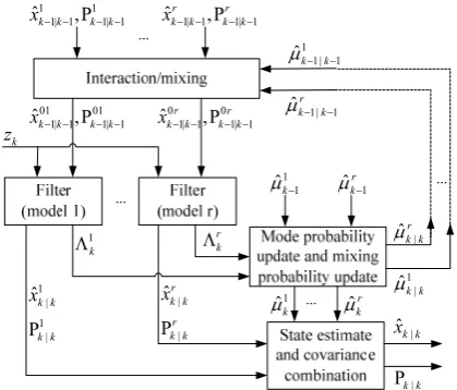
(42)In comparison to other MM estimators such as the generalized pseudo Bayes (GPB) method, only the step “interaction/mixing” is typical for the IMM estimator. A basic structure of the IMM is shown in Fig. 1.
Two standard IMM estimators, IMMEKF and IMMUKF, are derived when the nonlinear filtering
approaches such as the EKF and the UKF are used in the “filter” modules. A detailed implementation of the standard IMM filters refers to [5], [6].
B. Interacting Multiple Model Unscented Particle Filter Integrating a bank of unscented particle filters with the IMM method, an interacting multiple model unscented particle (IMMUPF) is derived. Starting from k-1, one cycle of the IMMUPF algorithm can be described in detail as follows.
(1) Interaction/mixing: Based on the Markov jump model, the model likelihoods and the posterior probability densities for different modes at k-1, the initial densities 0 0
1: 1 1
( | )
ˆ j j k k
p x− Z − are computed as Gaussian sum probability densities. The state estimate and covariance for each filter are initialized as
0 |
1| 1 1| 1 1| 1
1
ˆ
j rˆ
i i j,
k k k k k k
i
x
− −x
− −μ
− −=
=∑
(43)0 | 0 3
1| 1 1| 1 1| 1 1| 1 1| 1
1
ˆ
ˆ
P
j r i j{P
i[
i j][ ] },
Tk k k k k k k k k k
i
μ
x
x
− −
=
∑
= − − − −+
− −−
− −i
(44)where 0 1| 1
ˆ j k k
x− − andPk0− −j1|k 1 are the mixed initial condition
for mode-matched filter j at time k-1. Note that, in this context, i and j denote the corresponding model index respectively; n is the total number of sampling particles. Then the Gaussian mixing probabilities are computed via the equations:
|
1
1 1
1
,
i j i
ij k
k k
j
c
μ
− −=
π μ
− (45)1
1
,
r i
j ij k
i
c
π μ
−=
= ∑
(46)where cj is a normalization factor.
(2) State update/importance sampling: The sample set
1 1 1 1 1| 1 ,...,,..., , ,
|
{xˆk kj n− − ,Pk kj n− −}nj== rN is drawn from the state estimate 0
1| 1
ˆ j k k
x− − with the probability densities pˆk k0− −j1| 1 . Then,
propagate and update the sample set using the UPF to obtain the posterior samples 1
=1
, , , ,..., ,..., | P|
ˆ
{ j n, j n, j n n}j N r k k k k k
x w = at time
k, where j n, k
w is the normalized importance weight. At the same time, the mean of propagate output j
k
h ,
innovations j k
r , residual covariance Sˆkj and likelihood
functions j n, k
Λ can be calculated respectively as follows:
,
1
(
ˆ
, , ),
N j n
j
k k
n
h
h
k j
=
= ∑
x
(47),
ˆ
(
, , ),
j j n
k
=
k−
h
kk j
r
z
x
(48),
1
ˆ
j N[ (
ˆ
j n, , )
j][ ] ,
Tk k k
n=
h
k j
h
=
∑
−
i
S
x
(49),
(
,;0;
ˆ
).
j n j l j
k
N
k kΛ =
r
S
(50)(3) Residual resampling: Resample the sample set by evaluating the importance weights of all particles for each model to ensure the particles are distinct for an accurate posterior. The procedure, propagating the particles with
1 1
1| 1 1| 1
ˆk k ,Pk k
x− − − − xˆkr− −1| 1k ,Pkr− −1| 1k
k z | | ˆ P r k k r k k x 1 | 1 | ˆ P k k k k x
xˆk k |
|
Pk k
1
ˆk
μ ˆr k μ 1| 1 ˆr k k μ− − 1 1| 1
ˆk k μ− − 1 k Λ r k Λ 01 01
1| 1 1| 1
ˆk k ,Pk k
x− − − − ˆ01| 1,P01| 1
r r
k k k k
x− − − −
1 1
ˆk
μ− μˆkr−1
| ˆr k k μ 1 |
ˆk k μ
Figure 1. A basic structure of the standard IMM estimators.
higher-weights and suppressing the particles with lower- weights, is to generate a new sample set with identical
weights 1
1
, , ,..., ,..., |
ˆ
{xk kj n,wkj n=1/ }N nj== rN . A residual resampling
scheme is adopted for its smaller Monte Carlo variance and favourable computation time [20].
(4) Update of the mode probabilities:
,
1
,
j j n
j
k k
c
c
μ
= Λ
(51),
1
.
r j n
k j
j
c
c
=
=
∑
Λ
(52)(5) Estimate and covariance combination (output): Taking into account the mode probabilities, a combined state estimate can be obtained by averaging over the step 3 samples as follows:
, ,
| |
1
ˆ
,
r
n j n j n
k k k k k
j
x
x
μ
=
= ∑
(53)| |
1
1
ˆ
N n.
k k k k
n
x
x
N
==
∑
(54)The corresponding covariance is updated by the following equations:
, , ,
| | | |
1
ˆ
ˆ
P
n r j n{P
j n[
j n][ ] },
Tk k k k k k k k k
j=
μ
x
x
=
∑
+
−
i
(55)| |
1
1
P
NP .
nk k k k
n
N
==
∑
(56)V. SIMULATION AND ANALYSIS
To compare the performances of the IMMEKF, IMMUKF, IMMPF [18] and IMMUPF, a ground target tracking scenario is studied in this section. The four filters are then evaluated with the same sampling period of Δt=tk=1s. The tracking performance is chosen as the
root mean square errors (RMSEs). A. Scenario and Simulation Conditions
From the location of x=0km and y=1km, the target starts to make a positive CA movement for 54s with an initial velocity , initial acceleration and heading of 0m/s, 0.5m/s2 and 30o. Then it makes an almost CV motion for
162s. At last, the target makes a negative CA movement for about 54s with an acceleration of -0.5m/s2 until it
stops.
Remark 1: For an almost linear movement with an angle, it may be simplified the state dimensions through a coordinate rotation. But here in order to generalize the issue, we do not simplify this operation. Moreover, the measurements in a polar format may be converted to those in a Cartesian format through a coordinate conversion.
The mode transition matrix is given by
0.96 0.02 0.02
0.02 0.96 0.02 .
0.02 0.02 0.96
ijP
ijπ
⎡
⎤
⎢
⎥
=
= ⎢
⎥
⎢
⎥
⎣
⎦
(57)
The initial mode probabilities are set as 1 2 3
0 0 0 0.5
u = =u u = .
The standard deviations are taken to be: 1 1
ax ay
Q =Q =0.1 m2/s4, 2 2 2
ax ay
Q =Q = m2/s4 and 3 3 2
ax ay
Q =Q = m2/s4for the
process noise in the M1, M2 and M3 respectively; σr=2
m and σ =φ 0.001° for the measurement noise. For the IMMPF and IMMUPF approaches, the total particle number is set as N=600 with 200 particles for each model. B. Simulation
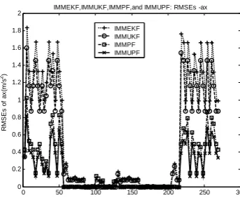
One hundred Monte Carlo simulations with different measurement noises to the same trajectory have been done. The RMSEs plots of each state vector for the four filters are shown in Fig. 2-7. A comparison of RMSEs over the whole period and the maneuvering phases and computational complexity for the four filters are shown in Table 1.
C Performance Analysis
(1) The estimate accuracy or RMSEs: It can be seen from Fig. 2-7 and Table 1 that the four filters perform almost the same in the non-maneuvering phase (between k=54s and k=216s); but in the maneuvering phase (before k=54s and after k=216s), the IMM particle filters outperform the standard IMM filters in reducing the state estimate errors. The reason is that the particle-type multiple model filters use the mixture of multiple Gaussians while the standard IMM filters use only single Gaussian mixing. Furthermore, the IMMUPF algorithm obtains more accurate estimates than the IMMPF algorithm because an UKF method is used to update the true mean and covariance of the proposal distribution.
(2) The computational complexity: It is an undeniable fact that the particle-type filters are computationally expensive. However, certain parallel mechanism in implementing the IMM-type filtering approaches (including the particle-type filters and IMM-type filters) can reduce the computational burden. Table 1 shows a comparison of total computational loads according to the CPU time (system configurations: Celeron (R) CPU 2.0 GHz, memory 512 MB). It can be seen from Table 1 that the standard IMM filters have better performance than the particle-type filters in the execution time.
VI. CONCLUSION
TABLE 1
A COMPARISON OF RMSES AND COMPUTATIONAL COMPLEXITY FOR THE FOUR FILTERS (100 RUNS, 3 MODELS)
Filters RMSEs (the whole period (k∈[1, 270])/the maneuvering phases(k∈[1, 54]∪[216, 270])) Total time(s) x (m) y (m) vx (m/s) vy (m/s) ax (m/s2) ay (m/s2)
IMMEKF 7.964/16.20 6.346/12.96 0.8216/1.883 0.6635/1.506 0.5575/1.304 0.4442/1.043 8.335 IMMUKF 6.970/14.22 5.524/11.376 0.6596/1.498 0.5176/1.168 0.4906/1.147 0.3127/0.9176 15.234
IMMPF 2.791/4.156 2.372/3.533 0.2447/0.4611 0.208/0.392 0.2127/0.504 0.1651/0.393 1.5823×10³ IMMUPF 2.271/3.419 1.960/2.905 0.174/0.2846 0.1427/0.233 0.1702/0.403 0.099/0.314 2.0965×10³
0 50 100 150 200 250 300 0
0.2 0.4 0.6 0.8 1 1.2 1.4 1.6 1.8 2
R
M
S
E
s
of
ax
(m
/s
2)
Time (s)
IMMEKF,IMMUKF,IMMPF,and IMMUPF: RMSEs -ax
IMMEKF IMMUKF IMMPF IMMUPF
Figure 6. A comparison of the four filters: RMSEs-ax.
0 50 100 150 200 250 300
0 0.2 0.4 0.6 0.8 1 1.2 1.4 1.6 1.8 2
R
M
S
E
s
of
ay
(m
/s
2)
Time (s)
IMMEKF,IMMUKF,IMMPF,and IMMUPF: RMSEs -ay IMMEKF IMMUKF IMMPF IMMUPF
Figure 7. A comparison of the four filters: RMSEs-ay.
0 50 100 150 200 250 300
0 0.5 1 1.5 2 2.5 3
R
M
SEs
o
f Vy
(m
/s
)
Time (s)
IMMEKF,IMMUKF,IMMPF,and IMMUPF: RMSEs -Vy IMMEKF IMMUKF IMMPF IMMUPF
Figure 5. A comparison of the four filters: RMSEs-vy.
0 50 100 150 200 250 300 0
0.5 1 1.5 2 2.5 3
R
M
SEs o
f
V
x
(m
/s
)
Time (s)
IMMEKF,IMMUKF,IMMPF,and IMMUPF: RMSEs -Vx
IMMEKF IMMUKF IMMPF IMMUPF
Figure 4. A comparison of the four filters: RMSEs-vx.
0 50 100 150 200 250 300 0
2 4 6 8 10 12 14 16 18 20
R
M
SE
s o
f x(
m
)
Time (s)
IMMEKF,IMMUKF,IMMPF,and IMMUPF: RMSEs - x
IMMEKF IMMUKF IMMPF IMMUPF
Figure 2. A comparison of the four filters: RMSEs-x.
0 50 100 150 200 250 300
0 2 4 6 8 10 12 14 16 18 20
R
M
SEs
o
f
y
(m
)
Time (s)
IMMEKF,IMMUKF,IMMPF,and IMMUPF: RMSEs - y IMMEKF IMMUKF IMMPF IMMUPF
ACKNOWLEDGMENT
This work was supported in part by the National Natural Science Foundation of China (No.60673024) and the National Defense Pre-research Plan of China.
REFERENCES
[1] Ronghua Guo, Zheng Qin, Xiangnan Li, and Junliang Chen, “An IMM Method to Ground Target Tracking,” The 2007 IEEE International Conference on Systems, Man, and Cybernetics (SMC 2007), Montreal , Canada, pp.96-101, Oct. 2007.
[2] L. Hong, N. Cui, M. Bakich, J. R. Layne, “Multirate interacting multiple model particle filter for terrain-based ground target tracking,” IEE Proceedings-Control Theory and Applications, vol. 153, no. 6, pp. 721-731, 2006. [3] C. Chong, D. Garren, T. P. Grayson, “Ground target
tracking--a historical perspective,” In: Proceedings of the IEEE Aerospace, Big Sky, MT, 2000.
[4] N. Cui, L. Hong, J.R. Layne, “A comparison of nonlinear filtering approaches with an application to ground target tracking,” IEEE Trans. Signal Processing, vol. 85, no. 8, pp. 1469-1492, 2005.
[5] Y. Bar-Shalom, S. Challa, H. A. P. Blom, “IMM estimator versus optimal estimator for hybrid systems,” IEEE Trans. on Aerospace and Electronic Systems, vol. 41, no. 3, pp. 986-991, 2005.
[6] Y. Bar-Shalom, Li Xiao-Rong, Estimation and tracking: principles, techniques, and software [M], Artech House, 1993.
[7] A. H. JAZWINSKI, Stochastic processes and filtering theory. Academic Press, New York, 1970.
[8] N. J. Gordon, D. J. Slamond, A. F. M. Smith, “Novel approach to nonlinear/non-Gaussian Bayesian state estimation,” IEE Proc. F, vol. 140, no. 2, pp. 107–113, Apr. 1993.
[9] R. van der Merwe, N. de Freitas, A. Doucet, E. Wan, “The unscented particle filter,” Technical Report CUED/ FINFENG/TR380, Engineering Department, Cambridge University, August 2000.
[10]R. van der Merwe, “Sigma-Point Kalman Filters for Probabilistic Inference in Dynamic State-Space Models,”
Ph.D. dissertation, Oregon Health Sci. Univ., Portland, OR, 2004.
[11]S. J. Julier, J. K. Uhlmann, “A new extension of the Kalman filter to nonlinear systems [A],” The Proc of AeroSense: 11th Int. Sym. posium Aerospace/Defense Sensing, Simulation and Controls[C]. Orlando, pp. 54-65, 1997.
[12]S. J. Julier, “The scaled unscented transformation,”
Proceedings of the 2002 American Control Conference, vol. 6, pp. 4555-4559, 2002.
[13]E.A. Wan, R.Van der Merve, “The unscented Kalman filter for nonlinear estimation [A],” Proc of Symposium 2000 on Adaptive Systems for Signal Processing, Communication and Control[C]. Lake Louise, Alberta, pp.153-158, 2000. [14]C. Musso, N. Oudjane, and F. Le Gland, “Improving
regularized particle filters” in A. Doucet, N. de Freitas, and N. Gordon, (Eds.): “Sequential Monte Carlo methods in practice” (Springer, New York, 2001), pp. 247–271. [15]S. McGinnity, G. W. Irwin, “Multiple model bootstrap
filter for maneuvering target tracking,” IEEE Trans. on
Aerospace and Electronic Systems, vol. 36, no. 3, pp. 1006-1012, July 2000.
[16]Y. Boers, and J. N. Driessen, “Hybrid state estimation: A target tracking application,” Automatica, 38, (12), pp. 2153–2158, 2002.
[17]N. J. Gordon, S. Maskell, and T. Kirubarajan, “Efficient particle filters for joint tracking and classification,” Proc. SPIE–Int. Soc. Opt. Eng., 4728, pp. 439–449, 2002 [18]Y. Boers, J. N. Driessen, “Interacting multiple model
particle filter,” IEE Proc.-Radar Sonar Navig., vol. 150, no. 5, pp. 344-349, Oct. 2003.
[19]Li Xiao-Rong; VP Jilkov, “Survey of maneuvering target tracking. Part I. Dynamic models,” IEEE Trans. on Aerospace and Electronic Systems, 4(39):1333-1363, 2003. [20]M. S. Arulampalam, S. Maskell, N. Gordon, T. Clapp, “A tutorial on particle filters for online nonlinear non-Gaussian Bayesian tracking,” IEEE Trans. Signal Processing, vol. 50, no. 2, pp. 174-188, 2002.
[21]W.H. Press, S.A. Teukolsky, W.T. Vetterling and B.P. Flannery, Numerical Recipes in C: The Art of Scientific Computing, Cambridge University Press, 2 edition, 1992. [22]C. P. Robert, G. Casella, Monte Carlo Statistical Method,
Springer-Verlag, New York, 1999.
[23]E Mazor, A. Averbuch, Y. Bar-Shalom, and J. Dayan, “Interacting multiple model methods in target tracking: a survey,” IEEE Trans. on Aerospace and Electronic Systems, vol. 34, pp. 103–123, 1998.
Ronghua Guo was born in Hubei Province, China. He
received his M.S. from Navy Engineering University in 2003 and now he is a Ph.D. candidate of Department of Computer Science & Technology, Tsinghua University, Beijing, China. His research interests include nonlinear control, particle filter and target tracking.
Zheng Qin is a Professor of the school of software, doctoral
mentor of department of computer science and technology, Tsinghua University, Beijing, China. His major research interest includes software architecture, data synthesis and nonlinear control. He has published dozens of research papers on key journals and conferences both at home and abroad, and some books as well.
Xiangnan Li received the B. Sc. degree from Hunan
University, Changsha, China in 2006. He is currently a M. S. student in Software of School, Tsinghua University, Beijing, China. His research interests include nonlinear control and target tracking.
Junliang Chen received the B. Sc. degree from Xi’an