Vehicle Routing Problem with Time Windows
for Reducing Fuel Consumption
Jin Li
School of Computer and Information Engineering, Zhejiang Gongshang University, Hangzhou, P.R.China
Email: jinli@mail.zjgsu.edu.cn
Abstract—Most of the studies on vehicle routing problem
with time windows (VRPTW) aim to minimize total travel distance or travel time. This paper presents the VRPTW with a new objective function of minimizing the total fuel consumption. A mathematical model is proposed to formulate this problem. Then, a novel tabu search algorithm with a random variable neighborhood descent procedure (RVND) is given, which uses an adaptive parallel route construction heuristic, introduces six neighborhood search methods and employs a random neighborhood ordering and shaking mechanisms. Computational experiments are performed on realistic instances which shed light on the tradeoffs between various parameters such as total travel distance, total travel time, total fuel consumption, number of vehicles utilized and total wait time. The results show that the solution of minimizing total fuel consumption has the potential of saving fuel consumption contrary to the solution of the traditional VRPTW, and is beneficial to develop environmental-friendly economies.
Index Terms—vehicle routing, time windows, fuel
consumption, tabu search, transportation
I. INTRODUCTION
Transportation has hazardous impacts on the environment, such as resource consumption, land use, acidification, toxic effects on ecosystems and humans, noise and Greenhouse Gas (GHG) emissions[1]. Among these, fuel consumptions are the most concerning as they not only are the main cost of the companies, but also cause serious pollution which has direct consequences on human health and environment. Rising fuel prices and growing concerns about GHG pollution of transportation on the environment call for revised planning approaches of road transportation to reduce fuel consumption. Our purpose is to introduce a new variant vehicle routing where optimizing the VRP by minimizing the fuel consumption.
The Vehicle Routing Problem (VRP)[2] aims at planning the routes of a fleet of vehicles on a given network to serve a set of clients under side constraints. The literature on the VRP and its variants is rich[3][4][5]. A common variant is the VRP with Time Windows (VRPTW) where the minimum-cost routes is found starting from and returning to the same depot that visits a set of clients once, each with a predefined time slot. Comprehensive surveys of solution techniques for the VRPTW can be found in Solomon[6] and Cordeau et
al.[7]. Figliozzi[8] proposed an iterative route construction and improvement heuristics for the VRP with soft time windows, which penalties are imposed to the total cost in case the client delivery time window can’t be met. Pang[9] presented a route construction heuristic with an adaptive parallel scheme. Yu and Yang[10] developed an improved ant colony optimization (IACO) to solve period vehicle routing problem with time windows, in which the planning period is extended to several days and each client must be served within a specified time window. Najera and Bullinaria[11] proposed and analyzed a novel multi-objective evolutionary algorithm, which includes methods for measuring the similarity of solutions, to solve the multi-objective problem.
The traditional objectives of the VRPTW focus on minimizing the total distance traveled by all vehicles or minimizing the total cost, which usually is a linear function of distance. It has been suggested by a number of studies that there are opportunities for reducing fuel consumption by extending the traditional VRP objectives to account for wider environmental and social impacts rather than just the economic costs[12]. But to minimize the vehicle’s travel distance does not necessarily produce the optimal solution from a fuel-efficiency standpoint. The reason is that the fuel consumption of a vehicle is affected not only by the travel distance, but also by other factors such as vehicle speed and road gradient in each segment [13][14].
Some related studies have taken into account energy consumption in vehicle routing from their own different perspectives. Kara et al.[15] introduced a so-called energy-minimizing vehicle routing problem which is an extension of the VRP where a weighted load function (load multiplied by distance) is minimized. Kuo[16] proposed a simulated annealing (SA) algorithm for finding the time-dependent vehicle routing with the lowest total fuel consumption. Suzuki[17] developed an approach to the time-constrained, multiple-stop, truck-routing problem that minimizes the fuel consumption and pollutants emissions.
factors, especially the fuel consumption during the wait time at clients’ sites. In VRPTW, the vehicle is often required to wait at clients’ sites because vehicle’s arrive may precede the start of time window. However, most studies have implicitly assumed that the fuel consumption during wait time is zero. The fact is that a vehicle may consume fuels during wait time for various reasons such as heating or cooling the driver’s compartment. So, we describe a comprehensive measurement approach of fuel consumption taking into account a broader and comprehensive factors including distance, speed, load and wait time, etc. Then, we define a minimal-fuel VRPTW model. To solve this problem, a novel tabu search algorithm with a Random Variable Neighborhood Descent procedure (RVND) is given. We also perform analyses using numerical examples to shed light on the tradeoffs between various performance measures of vehicle routing, such as distance, travel time and fuel consumption, assessed through a variety of objective functions.
This paper is organized as follows. The next section provides a formulation of minimal-fuel VRPTW. Section 3 describes the tabu search algorithm with RVND for the model. Computational experiments and analyses are presented in Section 4. The final section contains our conclusions.
II. FORMULATION OF MINIMAL-FUEL VRPTW
A. Prolbem Description
The minimal-fuel VRPTW can be defined as follows. Let G=(V, E) be a complete graph with V ={0,1,L,
}
n as the set of nodes and E={(i,j)|i,j∈V,i≠ j} as the set of arcs defined between each pair of nodes. Node 0 is the depot. There exists a homogeneous set of vehiclesK ={1,2,L,m}, each with capacityQ. Each edge (i,j)∈E has non-negative travel distance dij and travel time tij.Every client i∈V \{0} has demanddi, vehicle’s arrival time
a
i, wait timewi, service timesi, and a request to be served within a predefined time interval[ei,li].The objective is to find the optimal routes of minimizing the total fuel consumptions while meeting the overall client demands. The constraints include:
• Depot constraints: The vehicles start from and returning the only one depot.
• Vehicle’s capacity constraints: The total load a vehicle carries can’t exceed its capacity.
• Time window constraints: The vehicle is required to visit a client within a predefined time window. The vehicle is allowed to arrive before the opening of the time window, and wait until the client is available. But, the vehicle is not allowed to arrive after the close of the time window. So, this is a VRP with hard time window.
B. Measurement of Vehicle’s Fuel Consumption
We introduce a measurement of fuel consumption similar to Suzuki[17]. Let MPGij be vehicle’s miles per
gallon of fuel consumption in arc(i,j), and vij be the average speed in arc (i,j) . MPGij is expressed as a function of vij.
ij
ij v
MPG =α +0 α1 (1)
where α0≥0,α1≥0are the parameters to be estimated. Since the effect of vehicle speed on mpg based on long-time data, to compute the effect of vehicle speed on mpg for each arc based on the road gradient and load, we adjust (1) as:
ij ij ij
ij v
MPG =(α0+α1 )γ π (2)
where γij >0 is the parameter of the road gradient factor, which measures the deviation of a vehicle’s mpg in each arc from the standard, flat terrain value (γij =1represents
the flat terrain, γij<1 describes the positive gradient, and 1
> ij
γ is for the negative gradient), πij>0 is the parameter of load factor that measures the deviation of a vehicle’s mpg in each arc from the average value based on the load.
The effect of vehicle load on mpg can be expressed as a linear function: mpg=β0+β1L, where Lis the load,
0 0≥
β is the mpg of a vehicle when it is empty, β1<0 is the coefficient measuring the loss of mpg caused by additional load. So, we can describe πijas:
μ β β
β β π
1 0
1 0
+ + =
∑
∈Yij
i i
ij
d
(3)
where Yij⊆V\{0} is the client set unvisited when the vehicle is traveling on arc (i,j); and
μ
is the average load of the vehicle in the long run. Equation (3) indicates that when the load isμ
,π
ij =1; when it is less thanμ
,1 >
ij
π
; when it is larger thanμ
,π
ij <1.Let
ρ
≥0 denote the average amount of fuel consumed per hour while a vehicle is waiting at client sites. The fuel consumption at client i during the wait time is described as:WGPHi =wiρ (4) C. Proposed Formulation
According to the measurement of fuel consumption from (2) to (4), the formulation of minimal-fuel VRPTW is described as the following:
min
∑
∑
∈ ∈ ij E +
ijk ij ij ij ij K
k
x v
d
) ,
( (α0 α1 )γ π
+
∑
∈N\{0}
i i
w ρ (5)
} 0 { \ , 1
.
.t x j V
s
V i
ijk K k
∈ ∀ =
∑
∑
∈ ∈
} 0 { \ , 1 i V x V j ijk K k ∈ ∀ =
∑
∑
∈ ∈ (7) K k x x jk V j k i V i ∈ ∀ = =∑
∑
∈ ∈ , 1 0 } 0 { \ 0 } 0 { \ (8)∑ ∑
∑
∑
∈ ∈ ∈ ∈ = = Kk j V
jk V i k i K k m x x } 0 { \ 0 } 0 { \
0 (9)
2 | | }, 0 { \ ,
1 ∀ ⊆ ≥
≥
∑∑
∑
∈ ∈ ∈ S V S x Si j S
ijk K k (10) } 0 { \ ,
, k K i V x x V j jik ijk V j ∈ ∀ ∈ ∀ =
∑
∑
∈ ∈ (11) K k Q x d V j ijk i V i ∈ ∀ ≤∑
∑
∈ ∈ , } 0 { \ (12) K k j i V j i x a t s wai+ i+ i+ ij− j) ijk ≤0, ∀, ∈ , ≠ ,∀ ∈
(
(13)
V i l
ai≤ i, ∀ ∈ (14)
V i l w a
ei≤ i+ i≤ i, ∀∈ (15)
K k V j i
xijk∈{0,1}, ∀, ∈ ,∀ ∈ (16) where xijk is the set of decision variables, for each arc
) ,
(i j and vehicle k , xijk =1 if and only if the optimal solution, arc (i,j) is traversed by vehicle k and equal 0, otherwise.
The objective function is derived from (5) that measures the total fuel consumption of vehicle routing. Constraints (6) and (7) are constraints of visiting each client once. Constraints (8) and (9) are depot constraints. Constraints (10) are used to avoid sub-loop of the routes. Balance of flow is described through constraints (11). Constraints (12) are vehicle’s capacity constraints. Constraints (13)-(15) are time window constraints. Constraints (16) are the decision-variables constraints.
III. TABU SEARCH ALGORITHM
A. Framework of Algorithm
Tabu Search (TS) has been used to study the classical VRP and its variants[7], and presents better performance. So, we choose TS as our framework of algorithm. Compared with Genetic Algorithm (GA), Simulated Annealing (SA) and other metaheuristics, TS has faster searching ability and high quality of escaping the local optimum. However, TS is dependent on its initial solution. A better initial solution will help TS to search for a better solution. Meanwhile, given neighborhood structures usually restrict the stability and global search capability of the algorithm.
To conquer the shortcomings of TS, this paper presents an improved tabu search with RVND. Also, we introduce an adaptive parallel route construction heuristic (APRCH) [9] to construct the initial solutions. This algorithm can generate high quality initial solutions, and have been verified better than the common construction algorithms e.g. saving algorithms, insertion algorithms. We adopt random variable neighborhood descent procedure (RVND) which randomly selects a neighborhood operator to generate candidate solutions to change the fixed search
order and strength the ability of global optimization. The detailed steps of the algorithm are shown in the following.
Step 1: Initialization. The APRCH is used to construct the initial solutionX0. Suppose the maximum iteration
size is MaxOuterIter, and maximum iteration size of allowing the solutions not to be improved is MaxInnerIter. Set the neighborhood structures: the inter-route neighborhood set NL1={1-0, 1-1, 2-2, 2-opt*} and the
intra-route neighborhood set NL2 ={Or-opt, Reverse}.
CalculatingTF(X0), letX=X0, where X is the current
optimal solution.
Step 2: Local search. Performing the RVND based on current solution.
2.1. Selecting a neighborhood N∈NL1 randomly to
operate on current solution, and the best non-tabu solution X′ is obtained.
2.2. If TF(X′)<TF(X), the neighborhood operators in
2
NL are executed in sequence to further improve the solution; Select the best non-tabu solution as current solution, update the current optimal solution X , reset
1
NL , and go to step 2.1; otherwise update NL1=NL1\{N}.
2.3. IfNL1=φ, go to step 3, else go to step 2.1.
Step 3: Restarting and shaking. If the current optimal solution is not improved exceeding a given iterations size (MaxInnerIter), restarting is adopted on current optimal solution and the tabu list is cleared. To change the current search direction, three neighborhood operators are selected to execute from 1-0, 1-1, 2-opt*, 2-2, Or-opt, Reverse. Then, go to step 2.
Step 4: Evaluation of algorithm termination. If the maximum iteration size (MaxOuterIter) is reached, the algorithm is terminated and the optimal solution X∗ is output, else go to step 2.
B. Initial Solution Construction
The APRCH is designed to specifically construct the initial solutions for VRPTW. So, we construct the initial solution based on the idea of APRCH. This algorithm balances the effect of fuel consumption, time urgency and waiting time on route construction by assigning weights. It can adjust the weights of these three cost factors adaptively to gain the best route construction. When a vehicle k serves client j traveling through arc (i,j), the detail to calculate the cost factors below.
(1) Fuel consumption cost
Since the vehicle load is unknown before the route construction is completed, the load is not taken into account in fuel consumption cost to simplify the problems. ρ γ α α j ij ij ij ijk w v d f + + = )
( 0 1 (17)
(2) Time urgency cost
It is the time of vehicle k from the arrival time of client j to the latest opening service time as shown in Fig. 1.
) ( i i i ij
j
ijk l a w s t
Figure 1. Time urgency cost of client j.
(3) Waiting time cost
It is a waiting time when vehicle karrives at client j’s location.
)} (
, 0
max{ j i i i ij
ijk e a w s t
w = − + + + (19) We further define the Fitness measure as a weighted sum of the three factors by the weightsωd,ωu and ωw assigned to the fuel consumption, time urgency and waiting time cost factors respectively.
ijk w ijk u ijk d
ijk f u w
Fitness =ω +ω +ω (20) where ωd+ωu+ωw=1, ωd≥0, ωu≥0, ωw≥0.
The detailed steps of the algorithm are shown below.
Step 1: Calculate the lower bound on the number of vehicles required serving all clients based on total client demands and vehicle’s capacity by the ceiling function as follows:
⎥ ⎥ ⎥ ⎥ ⎥
⎥ ⎤
⎢ ⎢ ⎢ ⎢ ⎢
⎢ ⎡
=
∑
∈ Q
d
m iV
i
} 0 {
\ (21)
Define the initial step size sd,su,sw∈[0,1] of the weightsωd , ωu andωw , and search ranges[ld,μd] ,
] ,
[lu μu and [lw,μw]⊆[0,1]. Set step convergence factor
] 1 , 0 [ 1∈
λ and interval convergence factor λ2∈[0,1]. Given termination step size of the algorithm smin.
Step 2: Initialize m empty routes to the vehicle set R, without client assigned.
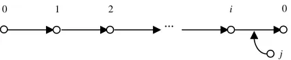
2.1. Select the location before the final node of the current route as the position the client is inserted into. For example, If the current route is (0,1,2,…,i,0), the position the client j is inserted into is shown in Fig. 2. Judge whether the clients unassigned to the routes are taken as candidate nodes to be assigned according to vehicle’s time and capacity constraints. If there are clients which can’t be assigned to any route, a new vehicle must be initiated to serve these clients. Then the route of the generated vehicle is added to R.
Figure 2. The position inserted by client j.
2.2. Let U be the set of clients unassigned to any route. For the route of vehicle kbelongs to R, calculate
}
min{Fitnessijk , ∀k∈R,∀j∈U, where the final client of the route is i. And Let the best client to be assigned to the corresponding vehicle.
2.3. Repeat steps 2.1-2.2 until U =φ . If the fuel consumption is reduced, update the current optimal solution which is the best solution found from the beginning to the current of the algorithm.
Step 3: Based on the current step sizes (sd,su,sw) and the search ranges ( [ld,μd] , [lu,μu] and [lw,μw] ), enumerate all the valid combinations of the weights
d
ω ,ωuan ωw. If a new better solution is found, adjust the search range so that the weights that give the best solution are located in the middle of the new search range, and recalculate the step size. If no better solution is found, reduce both the step size and the search range of the weights in terms of the convergence factors λ1 and λ2.
Repeat steps 2.1-2.3 until the step size is smaller than
min
s .
C. Local Search
We employ six VRP neighborhood structures[9][18], which are 1-0,1-1,2-2,2-opt*,Or-opt, and Reverse. The neighborhood operators including 1-0,1-1,2-2, and 2-opt* are inter-route neighborhoods, and the rest involving Or-opt and Reverse are intra-route neighborhoods. The route is encoded with natural numbers where the depot is denoted as 0 and the clients is represented as 1,2,…,n. Different with the traditional local search, the clients are operated with those neighborhoods under the conditions where vehicle’s capacity and time windows constraints must be met, and the objective function is reduced.
(1) 1-0, 1-1, 2-2. These are inter-route movements, also called Swap/Shift movements. 1-0, that is Shift (1,0), represents that a client from one route is inserted into another route. For example, the client 3 is moved from the route (0123450) to the route (067890) before client 8, which generates the route (012450673890). 1-1, that is Swap (1,1), performs permutation between a client from one route and a client from another route. For example, client 3 from the route (0123450) and client 8 from the route (067890) are swapped to gain the route (012845 067390). 2-2, that is Swap(2,2), means that two adjacent clients from one route are permutated by another two adjacent clients from other route. For example, the adjacent clients 2 and 3 from the route (0123450) are exchanged with the adjacent clients 7 and 8 from the route (067890) to obtain a route (017845062390).
(2) 2-opt*. It is the extension of Shift(1,0). This operator can realize permutation between adjacent tail clients from one route and adjacent tail clients from another route. For example, clients 3,4,5 from route (0123450) are exchanged with clients 8,9 from route (067890) to get a route (012890673450). The operator can also construct one route by connecting the tails of the two routes to reduce the number of vehicles, e.g. the tail of the route (0123450) is connected with the tail of the route (067890) to generate a route (01234567890).
(3) Or-opt. It is one of the intra-route neighborhood. One, two or three adjacent clients are removed and inserted in another position of the route. For instances, the clients 2 and 3 from the route (0123456780) are re-i
a ei
i
w si tij
j
a lj
ijk
u
t
0 1
…
i 0
inserted in the position before the client 7 to gain a route (0145623780).
(4) Reverse. This is also one of intra-route neighborhoods. This movement reverses the sub-route direction. For example, the client 2, 3, and 4 from the route (0123456780) had their direction reversed to form a route (0143256780).
In order to expand the search space, the depots are assigned based on the time and vehicle’s capacity constraints after the neighborhood operator is performed. For example, in the route (012345067890) which has been executed by one neighborhood, if the large demands of client 5 make the vehicle violate its capacity, the depots can be assigned according to the capacity constraints to generate the route (012340567890).
In these six neighborhood structures, the computational complexity of inter-route neighborhoods (1-0, 1-1, 2, 2-opt*) and Or-opt is O(n2) while the complexity of the neighborhood Reverse is O(n).
D. Restarting and Shaking
Restarting is to select a new solution as current solution to search. In this paper, the current optimal solution is selected as the restarting point. If the current optimal solution is not improved in a given iteration size , this optimal solution is taken as current solution while simultaneously clearing the tabu list to search solution space along a new direction.
To change the fixed search direction, shaking is applied to explore more solution space searching along a new direction. Here, shaking is used by performing three neighborhoods selected randomly from the six neighborhood structures (1-0, 1-1, 2-2, 2-opt*, Or-opt, Reverse).
IV. COMPUTATIONAL ANALYSIS
Experiments were run with data generated as realistically as possible. A transportation company that operating class-8 trucks plan delivery to clients. We randomly generate hypothetical, yet realistic, VRPTW instances. In each instance the problem specifications (dij,vij,tij,γij,di,ei,li,si)[17][19] are determined by random number operators as shown in table 1. We solve each instance using three models, which are minimal-distance model (denoted as FD) with minimizing the total travel distance, minimal-time model (denoted as FT) with minimizing the total travel time, and minimal-fuel model
(denoted as FF) with minimizing the total fuel consumption. Three classes of problems with n=10, 60 and 100 nodes are generated, where each class includes 10 instances and the experimental results is the average value of these 10 instances.
We describe some of the parameters for TS with RVND in the following: sd,su,sw =0.1; [ld,μd] =
] ,
[lu μu =[lw,μw]=[0,1]; λ1=0.01; λ2=0.01; smin =0.01;
MaxOuterIter=100; MaxInnerIter=10. All experiments are conducted on a PC with 1.58G Hz speed and 2Gb RAM. The TS algorithm with RVND is coded in Matlab 7.0. A common time-limit of 2 minutes was imposed on the solution time of all instances.
TABLE I. EXPERIMENTAL DATAS
Parameters Values (ranges)
Fixed Parameters
0
α (Speed regression intercept) 2.819632
1
α (speed regression slope) 0.065805 0
β (load regression intercept) 9.701
1
β (load regression slope) -0.00007491 ρ(fuel consumed per wit h) 0.3-0.9 gal. μ(average or base load) 33,451 lbs
i
s (service time at client) 0.1 h(all clients)
Q(vehicle’s capacity) 45,000 lbs
Random variables (specific to each experiment)
ij
γ (road gradient factor) 0.75-1.25
i
e (the earliest start service time) 8:00 am to 1:00 pm
i
l (the latest start service time) 2-6 h after ei
i
d (client demand) 5,000-10,000 lbs
ij
d (arc distance) 5-50 miles
ij
v (arc speed) 20-50 mph
ij
t (arc travel time) tij=dij/vij h
A. Effect of the Variation in Number of Nodes
This section presents the results of analyses in different number of nodes using the three different models (FD, FT and FF). Table 2 shows the five following measures obtained by the three models: total travel distance (TD), total travel time (TT), total fuel consumption (TF), the number of vehicles utilized (m), and total wait time (wt). All values are standardized to one for the FD objective.
TABLE II.
RESULTS OF EXPERIMENTS ON VARIOUS NUMBER OF NODES
n FT FF
TD TT TF m wt TD TT TF m wt
20 1.4243 0.7763 1.2739 1 0.3572 1.0614 0.9474 0.9472 1 0.9115
60 1.4373 0.7797 1.2934 0.9908 0.4155 1.0370 0.9392 0.9426 0.9908 0.9025
The figures shown in Table 2 makes it clear that there is no significant difference in the solutions yielded by models FT, FD and FF in terms of vehicles utilized where the average reductions in number of vehicles utilized using model FF is up to 0.31% than those produced by FD, and is up to 0.19% than those produce by FT. This shows that the TS with RVND can reduce the number of vehicles utilized to guarantee no significant difference in number of vehicles utilized. FF achieves an average reduction of up to 7.58% in total wait time than FD, but an average increase of up to 135.86% than FT. We can see that the fuel consumption during wait time is one of the factors that affect the total cost of fuel consumed, but does not play a leading role when ρ=0.7.
Some interesting implications of the results presented in Table 2 are as follows. Although the average total travel time and total wait time yielded by FT decrease by 22.40% and 60.65% respectively over those yielded by FD, the average total travel distance and total fuel consumption increase by 45.04% and 29.73% respectively, which suggests that the fuel consumption during wait time is not a dominating factor, and FD has better performance in saving fuel than FT. In addition, FT yields less number of vehicles utilized compared with FD (
n
=60 savings up to 0.92%,n
=100 up to 0.55%), which indicates that FT can save the number of vehicles utilized in contrast with FD.B. Effect of the Variation in Fuel Consumption during the Wait Time
This section presents the effect of the variation in waiting-time fuel consumption on various measures. The vehicle’s fuel consumption during the wait time is related with a number of factors such as vehicle types, air and so on. To this end, using a single 60-node instance, we have performed additional experiments when ρ=0.3, 0.5, 0.7, 0.9 as reported in Table 3.
The results presented in Table 3 suggest that as the waiting-time fuel consumption increases, the total fuel consumption grows, and the ratio of waiting-time fuel consumption to total fuel consumption is also increasing, e.g. the ratio is 7.77%, 11.97%, 15.34%, and 18.66% respectively. The reason is that as growing waiting-time fuel consumption, the waiting-time fuel consumption
becomes an important factor affecting the total cost of fuel consumption. So, to minimize the total fuel consumption, FF searches for the routes reducing the waiting-time fuel consumption, which decreases the waiting time.
We also note that FF achieves a significant fuel reduction over FD, and FF has a better fuel-saving performance (fuel-saving range increases from 4.23% to 5.89%) with increasing ρ , average fuel savings up to 5.07%. Since FT always finds the minimal total wait time, FT can save more fuel with increasing ρ , and the difference of FT, FF, and FD in fuel consumption becomes narrow, e.g. the range of fuel savings yielded by FF gradually decreases in comparison with those yielded by FT (decreasing from 35.94% to 27.21%). However, FF still has a average fuel reduction of up to 30.94% over FT. The analysis tells us that FF could obtain the most economical fuel-saving routes on various waiting-time fuel consumption.
Taking into account the number of vehicles utilized, FF is better than FD (average reduction up to 1.12%). FT can find the solution with minimal number of vehicles, especially can reduce more number of vehicles utilized (decreasing 1.79% in average) than FD.
C. Effect of the Variation in Time Windows
In this section, we present results of computational experiments to analyze the effects of different time window constraints. For this purpose, we use the distance data of a single 60-node instance with ρ=0.7. According to above results, the average maximum time of the tour is 6 hour, and the maximum interval of the time windows is selected as 6. Time windows are initially quite loose; they are chosen as randomly selected intervals of 90% of the maximum time interval. From this instance, 20 nodes are then randomly selected while simultaneously narrowing down the corresponding time windows by a factor of
δ
set in the range of 10-90% in increments of 20%. We ensure that the time windows are not tight enough to generate infeasible solutions. Results of this experiment are shown in Table 4.TABLE III
RESULTS SHOWING THE EFFECT OF THE VARIATION IN WAITING-TIME FUEL CONSUMPTION
ρ FT FF
TD TT TF m wt TD TT TF m wt
0.3 1.5302 0.7799 1.4950 1 0.3645 1.0611 0.9770 0.9577 1 0.9796
0.5 1.4840 0.7706 1.3793 0.9821 0.3774 1.0716 0.9629 0.9532 0.9821 0.9496
0.7 1.4832 0.7883 1.3446 0.9730 0.3903 1.0439 0.9853 0.9452 0.9910 0.9414
TABLEIV.
RESULTS OF EXPERIMENTS ON VARIOUS TIME WINDOW CONSTRAINTS
δ
FT FFTD TT TF m wt TD TT TF m Wt
0.1 1.5204 0.7466 1.2793 0.9818 0.3812 1.0581 0.9019 0.9448 0.9909 0.8568
0.3 1.4436 0.7665 1.2754 0.9820 0.4104 1.0600 0.9409 0.9498 0.9910 0.9028
0.5 1.5180 0.7871 1.2776 0.9908 0.4003 1.0246 0.9445 0.9544 1 0.9178
0.7 1.4489 0.7889 1.2968 0.9821 0.4092 1.0461 0.9615 0.9819 0.9911 0.9348
0.9 1.2647 0.8110 1.2836 0.9649 0.4807 1.0451 0.9625 0.9878 0.9825 0.9382
The results presented in Table 4 indicate that the fuel consumption increases with time windows narrowed-down. The fuel savings with FF are more apparent under loose time windows (
δ
=0.1-0.5) where the maximum fuel savings achieved by FF is 5.52% when δ=0.1 over those produced by FD, and is 26.15% when δ=0.1 over those yielded by FT. There is no significant difference in fuel consumption for models FT, FD, and FF under tightened time windows (δ
=0.7-0.9). The reason is that the feasible solution space becomes narrow with tightened time windows, and the selected routes are very limited.Moreover, as the time windows become tight the number of vehicles utilized increases. It is worth mentioning that the average reductions in number of vehicles using model FT is 1.09% compared to those produced by FF, and is 1.97% compared to those produced by FD, especially under tightened time windows the reductions in number of vehicles is significant. These results suggest that model FT can yield the solutions with minimal number of vehicles, and reduce the number of vehicles utilized as many as possible.
V. CONCLUSION
Study on VRPTW considering fuel consumption is crucial to the distribution operations of food logistics and cold chain logistics. By introducing the idea of reducing fuel consumption and protecting environment, a minimal-fuel VRPTW model, a variant of the well-known VRP, is proposed. We present a measurement approach of fuel consumption affected by many factors such as travel distance, load, speed, and waiting time, etc. Due to the model belonging to NP-hard problems, a novel tabu search algorithm with random variable neighborhood descent procedure is given. This algorithm uses adaptive parallel algorithm to generate high-quality initial solutions while the neighborhood structures adopt random variable neighborhood descent and the restarting and shaking mechanism are also introduced. Finally, a comparative study on distance model, minimal-time model and minimal-fuel model is performed by computational experiments.
Results of the computational experiments on realistic instances yielded the following important conclusions:
• The traditional objective of minimal travel distance or minimal travel time does not necessarily imply minimization of fuel. A
trade-off exists among travel distance, travel time and fuel cost. The minimal-fuel model provides a 6.20% improvement in fuel consumption over the minimal-distance model, but increases the travel distance by 3.84% on average. And it also reduces fuel consumption by 27.67% compared to minimal-time model, but increases travel time by 21.90% on average.
• A minimal-distance model has a better performance in saving fuel consumption than minimal-time model (average savings up to 6.63%), but minimal-time model can reduce the number of vehicles utilized, especially for the case with more nodes and tightened time windows (reduction of vehicles up to 3.51%).
• The minimal-fuel solution can significantly save the fuel consumption simultaneously reducing the pollutant emissions, especially when the number of nodes and waiting-time fuel consumption increase.
Concerning over global warming has grown, reducing the carbon emissions has become an important issue for all industries. Minimizing fuel consumption will become increasingly important in comparison with other criteria e.g. short travel distance or time. Also, there are a lot of opportunities for future research to present new models considering other factors e.g. heterogeneous vehicles, time-dependent speeds and random client demands, or to develop a more structural optimization strategy e.g. SA or GA algorithms, and thereby extend the results of the present researches.
ACKNOWLEDGMENT
The authors wish to thank the reviewers for their valuable comments. This work was supported in part by the National Natural Science Foundation of China (Grant No.71171178), Humanities and Social Sciences Foundation of Ministry of Education of China (Grant No. 12YJC630091), Zhejiang Provincial Natural Science Foundation of China (Grant No. LQ12G02007), and Zhejiang Provincial Commonweal Technology Applied Research Projects of China (Grant No.2011C23076).
REFERENCES
[1] T. Bektas, G. Laporte. “The pollution-routing problem,”
[2] G. Dantzig, J. Ramser, “The truck dispathing problem,”
Management Science, vol.6, no. 1, pp. 80-91,1959. [3] F. Li, B. Golden, E. Wasil, “The open vehicle routing
problem: Algorithms, large-scale test problems, and computational results,” Computers& Operations Research, vol.34, no.10, pp.2918-293, 2007.
[4] C.Y. Ren. “Research on single and mixed fleet strategy for open vehicle routing problem,” Journal of Software, vol.6,no.10,pp.2076-2081,2011.
[5] J.Q. Wang. “Efficient intelligent optimized algorithm for dynamic vehicle routing problem,” Journal of Software, vol. 6, no.11,pp.2201-2208,2011.
[6] M. M. Solomon, “Algorithms for the vehicle routing and scheduling problems with time window constraints,”
Operations Research, vol.35, pp.254-264, 1987.
[7] J.F. Cordeau, G. Laporte, and A. Mercier, “A unified tabu search heuristic for vehicle routing problems with time windows,” Journal of the Operational Research Society, vol. 52, pp.928-936, 2001.
[8] M.A. Figliozzi, “An iterative route construction and improvement algorithm for the vehicle routing problem with soft time windows,” Transportation Research Part C, vol.18, pp.668-679, 2010.
[9] K.W. Pang, “An adaptive parallel route construction heuristic for the vehicle routing problem with time windows constraints,” Expert Systems with Applications, vol. 38, no.9 pp.11939-11946, 2011.
[10]B. Yu, Z.Z. Yang, “An ant colony optimization model: The period vehicle routing problem with time windows,”
Transportation Research Part E ,vol.47, pp.166-181, 2011. [11]A.G. Najera, J.A. Bullinaria, “An improved multi-objective evolutionary algorithm for the vehicle routing problem with time windows,” Computers & Operations Research, vol.38, pp.287-300, 2011.
[12]A. Sbihi, R.W. Eglese, “Combinatorial optimization and green logistics,” 4OR: A Quarterly Journal of Operations Research, vol.5, no. 2, pp.99-116, 2007.
[13]E. Ericsson, “Independent driving pattern factors and their influence on fuel use and exhaust emission factors,”
Transportation Research Part D, vol. 6, no.5, pp.324-345,2001.
[14]K. Brundell-Freij, E. Ericsson. “Influence of street characteristics, driver category and car performance on
urban driving patterns,” Transportation Research Part D, vol.10, pp.213–229, 2005.
[15]I. Kara, B.Y. Kara, M.K. Yetis, “Energy minimizing vehicle routing problem”, In: Dress, A. Xu, Y. Zhu, B. (Eds.), Combinatorial Optimization and Applications,
Lecture Notes in Computer Science, vol. 4616. Springer, Berlin/Heidelberg, pp. 62–71, 2007.
[16]Y. Kuo, “Using simulated annealing to minimize fuel consumption for the time-dependent vehicle routing problem,” Computers & Operations Research, vol. 59, no.1, pp.157–165, 2010.
[17]Y. Suzuki, “A new truck-routing approach for reducing fuel consumption and pollutants emission,” Transportation Research Part D: Transport and Environment, vol.16 , no.1, pp.73-77,2011.
[18]A. Subramanian, L.M.A. Drummond, C. Bentes, et al., “A parallel heuristic for the vehicle routing problem with simultaneous pickup and delivery,” Computers& Operations Research, vol.37, pp.1899–1911, 2010. [19]US department of energy, “Office of energy efficiency and
renewable energy,” Transportation Energy Data Book, 28th ed. USDoE, Washington, DC., 2009.
Jin Li was born in Jiangsu province, China. He received the B.S. and M.S. degrees from Nanchang University, Nanchang, Jiangxi Province, China in 2004 and 2007 respectively. He received the Ph.D. degree in management science and engineering department, School of management, at Fudan University, Shanghai, China in 2010.
From July 2010 until now he works as an assistant professor in the Department of Management Science and Engineering, School of Computer Science and Information Engineering, Zhejiang Gongshang University, Hangzhou, Zhejiang Province, China. He has authored/coauthored more than 20 scientific papers. His research interests include logistics and supply chain management, system modeling and simulation, network optimization, and emergency management.