Smooth Harmonic Transductive Learning

Smooth Harmonic Transductive Learning

Ying Xie

, Bin Luo

, Rongbin Xu

, Sibao Chen

a _{Department of Computer Studies, Anhui University, Hefei 230601, China}

Email: [email protected]

b _{School of Computer Science and Technology, Anhui University, Hefei 230601, China} Email:{luobin,xurb 910,}@ahu.edu.cn [email protected]

Abstract— In this paper, we present a novel semi-supervised smooth harmonic transductive learning algorithm that can get closed-form solution. Our method introduces the unla-beled class information to the learning process and tries to exploit the similar configurations shared by the label distribution of data. After discovering the property of smooth harmonic function based on spectral clustering in classification task, we design an adaptive thresholding method for smooth harmonic transductive learning based on classification error. The proposed adaptive thresholding method can select the most suitable thresholds flexibly. Plentiful experiments on data sets show our proposed closed-form smooth harmonic transductive learning framework get excellent improvement compared with two baseline methods.

Index Terms— harmonic function, transductive learning, adaptive threshold

I. INTRODUCTION

In machine learning study, the most general annotation method is to adopt labeled data to train the classifier. Next annotate the unlabeled data using this trained classifier. If the trainning procedure does not use the unlabeled information, we call it insductive learning [1], [2], [3]. As we all known, labeled examples are time consuming and expensive to achieve, as they require the efforts of human labor. We only can achieve a small set of labeled data and a large set of unlabeled ones in real world. So, the trained classifier based on the small set of labeled data usually is not good enough for all data’s learning. How to improve the performance of using small part labeled information to annotate the unlabeled instances automatically is a important topic in classification task apparently.

Besides these inductive learning algorithms that purely explore the structure of labeled data, researchers have also well utilized data structure information from both labeled and unlabeled instances in the training procedure to enhance learning performance with limited number of labeled ones. It is transductive learning. Great success has been achieved in this area, such as [4], [5], [6], [7], [8], [9], [10].

After data classifier trainning, attention also has been drawn to how to select suitable threshold in the class labels prediction. It is generally thought that there is natural threshold in predicting class labels [11], [12], [13], [14], [15], [16], but we find it does not hold either

on center data or non-center data. We analysis the data structure and design an Adaptive Thresholding method for classification work.

In this paper, we propose a novel Smooth Harmonic Transductive learning with Adaptive Thresholding framework. Our framework is built upon semi-supervised learning. Given labeled and unlabeled data features, we construct the transductive harmonic objective function. Then we introduce the class information to the leaning process and exploit the similar configurations shared by the label distribution of data. We can get elegant final closed-form solution. We perform our new framework to do annotation task on six data sets. Over the most majority of these data sets, our new framework outperforms other two state-of-the-art methods.

We summarize our contribution as follows:

1) We propose a Smooth Harmonic Transductive method which has elegant formulation and closed-form solution to enhance the semi-supervised classification performance.

2) We discover the smooth harmonic function can capture class-wise data structure.

3) We propose a novel Adaptive Thresholding method based on classification work to deal with the difficulty of label assignment in classification problem.

This paper is organized as follows. Section II describes the detail of transductive learning setting we are studying. We study the property of smooth harmonic function and describe the objective function for classification. Based on this research, Section II designs an Adaptive Thresholding method to automatically search the exclusive thresholds for different classes, and introduces the entire framework of Smooth Harmonic Transductive learning with Adaptive Thresholding. Experiments in Section III show the excel-lent performance of our proposed framework on different labeled size data in classification task.

II. TRANSDUCTIVELEARNING

Given input data Xall ∈ Rp×n, Xall =

{Xtrain,Xtest}, where Xtrain = {x1, . . . , xl},

where Ytrain = {y1, . . . , yl},Ytest = {yl+1, . . . , yn}. yij = 1means the j-th data instance belongs to thei-th class, otherwise yij = 0.

A. Transductive learning setup

Two different settings can be found to formalize trans-ductive learning problem [17].

Setting 1: The full data sample Xall of n = l+u

instances is given. The learning algorithm further receives the labels of a training data setXtrain of sizel selected from Xall uniformly at random without replacement. Then the remaining u absent labels instances serve as a test data setXtest.

Setting 2: The training setXtrainand test setXtestare

both drawn i.i.d. according to some distribution D. The labeled set Xtrain and the unlabeled set Xtest are made available to the learning algorithm without their labels.

In our paper, we study Setting 2. Transductive regres-sion differs from the classical inductive regresregres-sion since the learning algorithm is given the unlabeled test exam-ples beforehand, we also can exploit the label information to improve its classification performance.

B. Smooth harmonic transductive learning

We assume a connected graph G = (V, E), nodes V corresponding to n data points, E set means edges between data points. Consideringn×nsymmetric weight matrixW= [wij]on the edges, we set the weight matrix as

wij =exp

(

−

d

∑

k=1

(xik−xjk)2 σ2

k

)

(1)

where xik is the k-th component of instance xi. xik represents the vector xi ∈R. σis legth scale parameter for each dimension. From Eq.(1), we can find the nearby data points in Euclidean space which are associated with large edge weight.

There is a real-valued functionf :V →Ron our graph G, then we can predict the class information of unlabeled data based on this real-valued function. Here, we thinkf as fi = yi, i = 1, . . . , l as class information of labeled data. In real scene, nearby data points have similar labels no matter labeled data or unlabeled data. So, we have this objective energy function

min

f J =

1 2

∑

ij

wij(f(i)−f(j))2 (2)

The minimum energy function Eq.(2) isharmonic. Har-monic function contains two properties [13]: (1)Lf = 0 on same class data points, and is equal tofuon unlabeled data points. L=D−Wis the combinatorial Laplacian, whereD =diag(di) is the diagonal matrix with entries di =

∑

jwij. (2) The value of f at each unlabeled data point is the average of f at neighboring data points:

f(j) = 1 dj

∑

i

wijf(i), j=l+ 1, . . . , n (3)

For simple, Eq.(3) can be represented as

f =Pf (4)

where

P=D−1W (5)

Because of the maximum principle of harmonic func-tion [18], f is unique and satisfies f(j) ∈ (0,1) j = l+ 1, . . . , n. Laplacian embedding can be viewed as an operator on the space of functions and it can be written as L = SST, where S is the matrix whose rows are shown by the vertices and whose columns are shown by the edges of W. Each column corresponding to an edge e = {u, v} has an entry 1/√du corresponding to u, an entry −1/√dv corresponding to v. So, we can consider

S as a “boundary operator” mapping “1-chains” defined on edges of a graph to “0-chains” defined on vertices [19]. Considering weight matrix Wcan specify the data manifold structure. We can use Laplacian property and weight similarity to balance the class information f.

In real world, we can achieve a small set of labeled data and a large set of unlabeled ones. This is a typical situation in many practical scenarios. Using labeled data to annotate the unlabeled ones is semi-supervised learn-ing. Motivated by the great success of semi-supervised learning, it is more reasonable to explore transductive learning’s additional discrimination information hidden in unlabeled instances.

The transductive classification task may be summarized as follows: Given a set of both labeled and unlabeled data instances, we wish to assign class labels to all the already available unlabeled data points. Unlike induction classification here all unlabeled Xtest data are available during training.

Separating the Xall = {Xtrain,Xtest}, Yall =

{Ytrain,Ytest}, Ytrain = {y1, . . . , yl} is class labels vector of labeled data. Suppose Ytest = {0, . . . ,0} is class labels vector of unlabeled data which we want to predict. The Smooth Harmonic Transductive learning’s objective function is

f =αPf+ (1−α)Lf (6)

Let

f =

  fl

fu



 (7)

whereflrepresents the class information of labeled data, fu represents the class information of unlabeled data. In real world, we set α = 0.9 for using P information mainly.

Because data contain labeled and unlabeled informa-tion, we splitPinto four parts (similarly LandW),

P=



 Pll Plu

Pul Puu



Then, the harmonic function subject tof|L=fl is given by

  fl

fu

 =α



 Pll Plu

Pul Puu

 

  fl

fu



 (9)

+(1−α)



 Lll Llu

Lul Luu

 

  fl

fu



 (10)

We can get

fu=A−1Bfl (11)

where

A=I−αPuu−(1−α)Luu (12)

and

B=αPul+ (1−α)Lul (13)

Harmonic function is closely related to the random walk method [20]. On the graph G, a particle can walk start from unlabeled node i, then goes to node j with probability Pij after one step. When the particle hits a labeled data, the walking stop. In random walk, labeled data can be viewed as “absorbing boundary” [13].

Here, we use spectral clustering method to smooth the harmonic function, classical normalized cut approach [21] based on f is the minimization of the Raleigh Quotient

R(f) = f

T_Lf

fT_Df =

∑

ijwij(f(i)−f(j))2

∑

idif(i)2

(14)

This Raleigh Quotient’s solution is the second smallest eigenvector of Lf = λDf. So, data points can be clustered in the eigensystem spanned by the eigenvectors of L [22].

C. Adaptive thresholding

Taking account the actual data and appropriate thresh-olding, we propose an Adaptive Thresholding method for classification work. These Adaptive Thresholding values are varied in different datasets and even distinct in differ-ent classes of the same dataset.

The key idea of Adaptive Thresholding is that the classifier can also be used to predict class labels for each training data points whose true labels are known. These predicted values are not exactly{0,1}, so a threshold can be learned from the training data. In addition, because the training dataset and the test dataset have similar data distribution, our proposed method should work well after threshold h is also learned from the ground truth and predicted results of the training dataset.

During the learning of the threshold value, a criterion is needed. We present them as below.

Let bk as the adaptive decision boundary, S+ is the

number of positive samples for the k-th class, S₋ is the number of negative samples, so lete+(bk)ande−(bk)be the numbers of misclassified positive and negative training samples. Wang [23] used Bayes rule method to decide the

boundary. Here, we design the decision boundary based on smooth Bayes rule:

h∗_k = arg min

bk

(

αe+(bk)

|S+| + (1−α) e₋(bk)

|S−|

)

(15)

Based on Eq.(15), we can assign class labels to unlabeled data by:

ξij=

{

1 if yij > h∗k

0 if yij ≤h∗k

(16)

D. The framework of Smooth Harmonic Transductive learning

According to the above analysis, combining with S-mooth Harmonic Transductive function and Adaptive Thresholding, we introduce an accompany framework of v-fold cross validation classification as Algorithm 1. After getting the fu = Ytest, we use Adaptive Thresholding Method to analysis the class information.

We use v-fold cross validation to perform Smooth Harmonic Transductive learning and get the most rep-resentative index in Ytest to stand for class labels.

We will show the classification’s performance of S-mooth Harmonic Transductive learning and Adaptive Thresholding in Section III.

Algorithm 1The Smooth Harmonic Transductive

Learn-ing Framework UsLearn-ing Adaptive ThresholdLearn-ing

Input:

Xtrain = (x1, x2,· · · , xl)∈Rp×l

Ytrain = (y1, y2,· · ·, yl)∈Rk×l

Xtest = (xl+1, xl+2,· · ·, xn)∈Rp×u Initialization:

Center data Xtrain into X˜train. Center data Ytrain into Y˜train.

Fix the fold number of cross validation v. Randomly select the v-cross validation instances. Compute:

Compute combined matrix Pas Eq.(5).

Split P into four parts to separate train parts and test parts as Eq.(8).

Compute the fu as Eq.(11).

Compute the classification thresholdshusing Adaptive Thresholding based on Eq.(15).

Compute the classification accuracyaccusing Eq.(16). Output:

fu = Ytest ∈ Rk×u, thresholds h, classification accuracy acc.

III. EXPERIMENTS

A. Data sets description

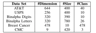
We adopt six data sets to verify our framwork. The detail of data sets shows in TABLE I. The data sets we select are plentiful and powerful to certificate our framework.

TABLE I.: The detail of data sets using in experiments.

Data Set #Dimension #Size #Class AT&T 644 400 40

USPS 256 400 10

Binalpha Digits 320 390 10 Binalpha Letters 320 780 26 Breast Cancer 478 10 478

CMC 9 420 3

B. Smooth harmonic transductive learning performance

We do Smooth Harmonic Trandsductive learning(SHT) of Eq.(11) on six data sets. The compared methods are f uHarmo and f uCM N [13]. f uHarmo method is fu= (I−Puu)−1Pulfl.f uCM N method is class mass normalization method to adjust the class distribution to match the priors. This method scales masses so that an unlabeled point iis classified as class 1 iff

q∑fu(i) ifu(i)

>(1−q)∑1−fu(i)

i(1−fu(i))

(17)

TABLE II shows the performance of 5-fold cross validation classification accuracy. Binalpha Digits data set gets the most great improvement on 5.56%. USPS data set get 3.95% improvement. Abalone data set get 3.66% improvement.

TABLE II.: Results of 2-fold cross validation classifica-tion using smooth harmonic transductive learning.

Data Set fuHarmo(%) fuCMN(%) SHT(%) AT&T 76.7 81.3 77.9

USPS 83.3 81.3 84.6

Binalpha Digits 62.0 74.5 65.0 Binalpha Letters 52.1 75.4 55.0 Breast Cancer 96.8 96.5 96.6

CMC 40.8 41.3 42.5

Our proposed method can get better classification re-sults than unsmooth f uHarmo method. In AT&T da-ta set, SHT method gets 1.56% improvement. Also in USPS data set. In Binalpha Digits, SHT can get 4.8% improvement. In Binalpha Letters, SHT can get 5.6% improvement. CMC can get 4.2% improvement.

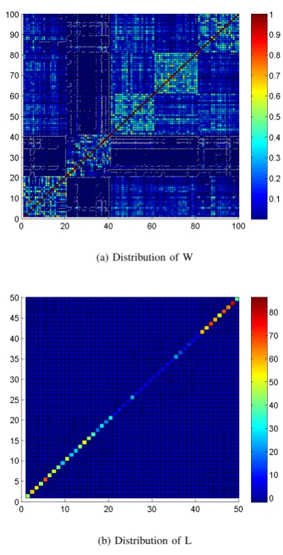
We also do experiments to test the performance under different labeled data size. Figure 1 to 6 show the results of six data sets. We can discover from these figures that in AT&T data set, our proposed SHT method is better than f uHarmo method before 50% data are labeled. When labeled data set size gets larger and larger, our SHT method is better than f uCM N method. In all six data sets, we can find the regular pattern. Because our proposed SHT method can explore transductive learn-ing’s additional discrimination information hidden in the unlabeled instances, it can capture class-wise structure Figure7. Then this method can improve the classification performance.

10 20 30 40 50 60 70 80 90

0.1 0.2 0.3 0.4 0.5 0.6 0.7 0.8 0.9 1

Labeled Data Set Size(%)

Classification Accuracy

fuHarmo fuCMN fuSHT

Figure 1: AT&T data set classification accuracy Decided by SHT based on different labeled data size.

10 20 30 40 50 60 70 80 90

0.2 0.3 0.4 0.5 0.6 0.7 0.8 0.9 1

Labeled Data Set Size(%)

Classification Accuracy

fuHarmo fuCMN fuSHT

Figure 2: USPS data set classification accuracy decided by SHT based on different labeled data size.

10 20 30 40 50 60 70 80 90

0.1 0.2 0.3 0.4 0.5 0.6 0.7 0.8 0.9

Labeled Data Set Size(%)

Classification Accuracy

fuHarmo fuCMN fuSHT

10 20 30 40 50 60 70 80 90 0

0.1 0.2 0.3 0.4 0.5 0.6 0.7 0.8

Labeled Data Set Size(%)

Classification Accuracy

fuHarmo fuCMN fuSHT

Figure 4: Binalpha Letters data set classification accuracy decided by SHT based on different labeled data size.

10 20 30 40 50 60 70 80 90

0.94 0.945 0.95 0.955 0.96 0.965 0.97 0.975 0.98 0.985

Labeled Data Set Size(%)

Classification Accuracy

fuHarmo fuCMN fuSHT

Figure 5: Breast Cancer data set classification accuracy decided by SHT based on different labeled data size.

10 20 30 40 50 60 70 80 90

0.35 0.4 0.45 0.5 0.55

Labeled Data Set Size(%)

Classification Accuracy

fuHarmo fuCMN fuSHT

Figure 6: CMC data set classification accuracy decided by SHT based on different labeled data size.

(a) Distribution of W

(b) Distribution of L

Figure 7: Distribution of two terms of SHT method.

IV. RELATEDWORK

A. Local Transductive Regression

LRT algorithms can be viewed as a series of the so-called kernel regularization-based learning algorithms to the transductive settings. The objective function is:

min

f J =||f||

2

K+α l

∑

i=1

(f(xi)−y(xi))2+β u

∑

i=1

(f(xi)−y˜(xi))2

(18) where || · ||K is the norm in the reproducing kernel Hilbert space(RKHS) with associated kernel K, α ≥ 0 andβ ≥0 are trade-off parameters, f is the hypothesis and(f(x)−y˜(x))2_{is the error off on the unlabeled point}

xwith respect to a pseudo-target y.˜ y˜is achieved from k-neighborhood labels y(x)by a local weighted average or other regression algorithms applied locally.

method and the labels from different classes could thus be employed to pilot the regression. Manifolds con-structed from different classes are regularized separately and utilize the inter-manifold relations. [8] proposed an approach that exploited a censored instance’s own partial information of true outcome rather than its neighbors’ labels to transduce optimal target times.

B. Unconstrained Regularization Transductive Regres-sion

Another family of transductive regression algorithms that can be formulated as the following optimization problem:

min Ypre

YT_preQYpre+(Ypre−Yall)TC(Ypre−Yall) (19)

where Q ∈Rn×n _{is a symmetric regularization matrix,}

C ∈ Rn×n _{is a symmetric(often a diagonal) matrix of} empirical weights,Yall∈Rk×nis the target values of the n labeled data instances together with the pseudo-target values of the u unlabeled data instances, and Ypre ∈

Rk×n _{is a matrix whose i-th row is the predicted target} value forxi. The close-form solution of Eq.(19). is given by

Ypre= (C−1Q+I)−1Yall (20)

This formulation is quite general and includes the algo-rithms of [11], [12], [13]. [14] designed an algorithm simultaneously learned the order of the decision bound-aries. At the same time the pseudolabels of unlabeled data with the decision boundaries were enforced to fall on low-density regions of both labeled and unlabeled data while satisfying the cluster assumption. [15] developed a statistical learning theory to demonstrate this aspect with regard to Transductive Support Vector Machine’s generalization ability.

C. Constrained Graph Regularization Transductive Re-gression

These methods define a weighted graph G = (Xall, W), edge W can be interpreted as similarity weights between vertices. The input space Xall is thus reduced to the set of vertices, and a hypothesis h : Xall → R can be identified with its predictions h =

[h(x1), . . . ,h(xn)]T. The hypothesis setH can thus be identified with Rl. So the task is predicting the vertices’ labels. Let htrain denote the restriction of h to the training points, [h(x1),· · ·,h(xl)]T ∈Rl, and similarly

letYtrain denote[y1,· · · , yl]T ∈Rl. The general family

of constrained graph regularization algorithms can then be defined by the following optimization problem:

min htrain

hTLh+α(htrain−Ytrain)T(htrain−Ytrain)

s.t.hTu= 0 (21)

where L ∈ Rn×n _{is the graph Laplacian matrix. L} is a positive semi-definite symmetric matrix. hT_{Lh =}

∑l

ij=1wij(h(xi)−h(xj))2. u ∈ Rn is a fixed vector

always defined to be all its entries equal 1. This con-straint of the objective function thus restricts the space of solutions to be inH1, the hyperplane inH of the vectors

orthogonal tou. It also definePas the projection matrix over the hyperplane H1 [16], [24].

Then, the Lagrangian associated to the objective func-tion Eq.(21) is

L=hTLh+α(htrain−Ytrain)T(htrain−Ytrain)+βhTu (22) whereβ ∈Ris a Lagrange variable. From the Lagrange function, we can get

∂L/∂h=Lh+α(htrain−Ytrain) +βu= 0 (23)

Multiplying by the projection matrix Pgives

P(L+αI)h=αPYtrain (24)

So, the solution of Eq.(21) is

htrain = [P(L α) +I]−1PYtrain (25) To the best of our knowledge, this is the first work to get closed-form solution in smooth transductive learning.

V. CONSLUSION

In this paper, we present a novel algorithm dedicated for the closed-form transductive learning problem. Infor-mation constructed from labeled and unlabeled data are regularized appropriately and utilize the unlabeled data’s classes information, we develop an efficient method and unlabeled data’s feature which can thus be employed to pilot the learning. The method puts the class labels information to the learning procedure and discovers the similar structure shared by the label distribution of data. Moreover, we design an Adaptive Thresholding method which can select suited class labels automatically. This Adaptive Thresholding is based on classification error. Plentiful experiments demonstrate the superiority of our proposed framework over the two state-of-the-art classi-fication algorithms.

ACKNOWLEDGMENT

The research is supported by the National Natu-ral Science Foundation of China(No.61202228). The International Cooperation Program of China (Grant No.2011DFA10850), the National Youth Fond of China (Grant No.61203290), the Teaching Project of Quali-ty Engineering in Anhui UniversiQuali-ty (JYXM201291 and JYXM201247).

REFERENCES

[1] J. Zhang and J. Huan, “Inductive multi-task learning with multiple view data.” inKDD, 2012, pp. 543–551. [2] K. Hovsepian, P. Anselmo, and S. Mazumdar, “Supervised

inductive learning with lotka-volterra derived models.” 2011, pp. 195–223.

[4] M. Belkin, I. Matveeva, and P. Niyogi, “Regularization and semi-supervised learning on large graphs.” inCOLT, 2004, pp. 624–638.

[5] X. Zhu and A. B. Goldberg, “Semi-supervised regression with order preferences,” Technical Report TR1578, Dept. of Computer Sciences, University of Wisconsin-Madison, Tech. Rep., 2006.

[6] C. Cortes, M. Mohri, and M. Mohri, “On transductive regression.” inNIPS, 2006, pp. 305–312.

[7] H. Wang, S. Yan, T. S. Huang, J. Liu, X. Tang, and X. Tang, “Transductive regression piloted by inter-manifold relations.” inICML, 2007, pp. 967–974. [8] F. M. Khan, Q. Liu, and Q. Liu, “Transduction of

semi-supervised regression targets in survival analysis for medi-cal prognosis.” inICDM Workshops, 2011, pp. 1018–1025. [9] Y. Guo and D. Schuurmans, “Semi-supervised multi-label classification - a simultaneous large-margin, subspace learning approach.” inECML/PKDD (2), 2012, pp. 355– 370.

[10] D. Kong and C. H. Q. Ding, “Maximum consistency preferential random walks.” in ECML/PKDD (2), 2012, pp. 339–354.

[11] M. Wu, B. Scho¨lkopf, and B. Scho¨lkopf, “Transductive classification via local learning regularization.” 2007, pp. 628–635.

[12] D. Zhou, O. Bousquet, T. N. Lal, J. Weston, B. Sch¨olkopf, and B. Scho¨lkopf, “Learning with local and global consis-tency.” inNIPS, 2004.

[13] X. Zhu, Z. Ghahramani, J. D. Lafferty, and J. D. Lafferty, “Semi-supervised learning using gaussian fields and har-monic functions.” inICML, 2003, pp. 912–919.

[14] C.-W. Seah, I. W. Tsang, Y.-S. Ong, and Y.-S. Ong, “Transductive ordinal regression.” 2012, pp. 1074–1086. [15] J. Wang, X. Shen, and W. Pan, “On transductive support

vector machines,” Contemporary Mathematics, vol. 443, p. 7, 2007.

[16] C. Cortes, M. Mohri, D. Pechyony, A. Rastogi, and A. Rastogi, “Stability analysis and learning bounds for transductive regression algorithms,” 2009.

[17] V. Vapnik, “Statistical learning theory.” 1998, pp. I–XXIV, 1–736.

[18] P. G. Doyle and J. L. Snell, Random walks and electric networks. Math. Ass. of America, 1984, vol. 22. [19] F. R. Chung, “Spectral graph theory (cbms regional

con-ference series in mathematics, no. 92),” 1997.

[20] M. Szummer and T. Jaakkola, “Partially labeled classifi-cation with markov random walks.” in NIPS, 2001, pp. 945–952.

[21] J. Shi and J. Malik, “Normalized cuts and image segmen-tation.” 2000, pp. 888–905.

[22] A. Y. Ng, M. I. Jordan, and Y. Weiss, “On spectral clustering: Analysis and an algorithm.” inNIPS, 2001, pp. 849–856.

[23] H. Wang, H. Huang, and C. H. Q. Ding, “Image annotation using multi-label correlated green’s function.” in ICCV, 2009, pp. 2029–2034.

[24] M. Belkin, P. Niyogi, and P. Niyogi, “Semi-supervised learning on riemannian manifolds.” 2004, pp. 209–239.

Ying Xieis currently a Ph.D student in Computer Application from Anhui University (Hefei,China), and at the same time she is a lectuer in Anhui University (Hefei, China). She received her Master degree in Computer Science from Anhui University, in 2008. Her current research interests include, but are not limited to, Machine Learning and Social Network.

Bin Luo is at present the dean and a professor of the School of Computer Science and Technology, Anhui University, China. He received his BEng degree in electronics and MEng degree in computer science from Anhui university of China in 1984 and 1991, respectively. In 2002, he was awarded the Ph.D. degree in Computer Science from the University of York, the United Kingdom. He was a research associate of the University of York, short term research fellow of British Telecom., UK, visiting fellow of the University of New South Wales, Australia, visiting professor at the Florida Institute of Technology, USA, visiting professor at the University of Stirling, UK. At present, he is holding a position of TCT Exchange Fellowship at Nanyang Technological University, Singapore.

He has published more than 200 research papers in journals, edited books and refereed conferences. Some of them were published on IEEE T-PAMI, Pattern Recognition, CVPR, IJCAI, AAAI. His research interests include graph models for image representation, image and graph matching, graph spectral analy-sis. He chairs the IEEE Hefei Subsection and is a senior member of IEEE. He is an associate editor of the journal of Cognitive Computation.

Rongbin Xu is currently a Ph.D student and a lectuer with the Faculty of Computer Science, Anhui University (Hefei, China). He received his master degree in Computer Science from Anhui University, in 2007. His current research interests include, but are not limited to, Image Processing, Cloud Computing, Scientific and Business Workflow. he is the corresponding author of the paper.