Analysis of Medical Image Pre-Processes of
Selected Magnetic Resonance Images
S Gamalendira1, Shilpa Singh2
1
College of Engineering, Design and Physical Sciences, Brunel University London, United Kingdom
2
Assistant Professor, Department of Radiology, Faculty of Allied Health Sciences, SGT University, Gurgaon,
Abstract: The medical image processing is one of the most challenging procedures, as it deals with the diagnosis of pathology and treatment is planned accordingly. MRI and other imaging modalities have become the most effective advanced technique in the medical sector thus it requires high accuracy and computational capabilities. Because of this reason the image processing techniques are crucial to enhance image quality in order to diagnose pathology accurately. Pre-processing is the most important step in the MRI image analysis due to poor captured MRI image quality and it is also very important to correct and adjust the MRI image for further subsequent steps of image processing. There are different types of techniques available for pre-processing such as filtering. Filters are applied on raw data to improve image quality, noise suppression, contrast enhancement, intensity equalization, outlier elimination, bias compensation, time/space filtering remove the noise, preserves the edges within an image, enhance and smoothen the image. This report evaluates the different types of pre-processing methods by the use of commercially available MATALB.
Key words: MRI, Preprocessing, Gaussian Filter, Mean Filter, Histogram Equalization
I. INTRODUCTION
Medical image seeks to investigate internal viscera of the body to diagnose the disease. But due to unwanted interference and other conditions it affects the measurement procedure in imaging and data acquisition system [1]. It is well known that the data acquisition method is specific for each technique and system; the magnetic resonances images are acquired in the different technique form other image modalities such as conventional X-ray and computed Tomography. It characterizes and differentiates the tissues based on their composition of hydrogen atoms, blood flow, cerebrospinal fluid flow, contraction and relaxation of organs and both physiologic and pathologic conditions [2].
However, the quality of Magnetic Resonance Image depends on various factors such as spatial resolution & image contrast, signal to noise ratio and artifacts [3]. Therefore there should be a procedure to minimize the effects of factors which influence on the quality of images, so the restoration of images tries to reduce the effects of these defects by the filters [4].
The basic idea in the image processing is the improvement of the image quality through the reduction of the noise. It requires a great variety of techniques dedicated to carry out this procedure. Each technique depends on the types of the noise in the images [5]. In the MRI, the noise is generally due to the rising electrical current and/ or eddy current in the wires of the gradient magnets being opposed by the main magnetic field. The stronger the main field, the louder the gradient noise [6].
Artifacts are also big challenges on quality of image as it may lead to misinterpretation of image or may mimic pathology. In medical imaging techniques, artifacts cannot be limited with few parameters because it is related from the equipment to the patient. These different types of artifacts can be assessed and solutions can be found to correct them [7].
Almost all the initial data of images are noisy, and some of the data is not clear enough to visualize. Therefore preprocessing plays an important role in the image quality and processing. Artifacts are common in the MRI and it could be created by patient or/and equipment. Patient related artifacts include motion beam hardening and metal artifact. Equipment related artifacts include partial volume effect, ghosting and staircase artifacts. Therefore it should be removed by any of the pre-processing procedures before proceeding to image reconstruction [8]. There are number filtering methods that have been identified to solve this problem [9].This report investigated some of the filters.
II. METHODOLOGY
Figure 1 Axial image of human artery-T1W Figure.2 Axial image of human artery-T2W
A. Gaussian filter
This filter works based on Gaussian function [10]. Gaussian filter is used to limit input with time. Commonly Gaussian filters are functioning as smoothing the output [11]. Following code is typical Gaussian filter’s code edited to analyze the images (Figure 1and Figure 2), based on consideration of the image, the file name of the image can be changed on the second line of code either Figure 1 or Figure 2.
clear all; close all;
im=imread('Figure 1'); %% read the image delta = 2;
G=Gaussian2D(delta); %% the filter kernel im1=filter2(G,double(im)); %% convolution im1=uint8(im1);
%% image show subplot(1,2,1); imshow(im) subplot(1,2,2); imshow(im1)
Where (delta) is the standard deviation of the pixel distribution, the distribution is assumed to have a mean value of 0. Normal distribution bell shaped curve represents Gaussian distribution, where a large value of produces a flatter curve, and a small value leads to a “pointier” curve [12].
B. Mean filter:
The mean filter replaces the center value of the frame with mean value of the entire pixel in the frame [13]. Following code is typical mean filter’s code edited to analyze the images as seen in figure 1 and figure 2, based on consideration of the image, the file name of the image can be changed on the second line of code either figure 1 or figure 2.
clear all; close all; im = imread('Figure 1'); h = fspecial('average', 11); im1=filter2(h,double(im)); im1 = uint8(im1);
[image:3.612.327.512.83.251.2]C. Histogram and Histogram Equalization
The histogram of an image normally refers to a histogram of the pixel intensity values. For an 8-bit gray scale image there are 256 different possible intensities, thus the histogram will graphically display 256 numbers showing the distribution of pixels amongst those gray scale values. Therefore the histogram plays an important role in representation of the pixels versus brightness of an image [14]. Histogram equalization is commonly used technique for image contrast enhancement. This technique assigns uniform distribution of intensity value of pixel for the output image [15]. Following code is typical Histogram code edited to analyze the images as seen in figure 1 and figure 2.
%%function for histgram function H = histogram_bru(I) %H the vector of histogram I = uint8(I);
H(1:256)=0; size_I = size(I); for i = 1 : size_I(1) for j = 1 : size_I(2) H(I(i,j)+1)=H(I(i,j)+1)+1; end
end figure; bar(H, 'b');
III. RESULTS AND DISCUSSION
The technique of every process is different from other because every technique has its own function and different outcome. In this series of images the one on right side always represents original image and the other one represents preprocessed image
[image:4.612.64.523.420.697.2]A. Gaussian filter
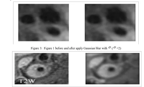
Figure 3: Figure 1 before and after apply Gaussian blur with
(
=2)Figure 3 and figure 4 compare the different image qualities before and after applying Gaussian smoothing filter. It is observed there are blurred images generated by this function; it replaces each pixel by linear combinations of its neighbors. In both the figures, the effect of smoothing is shown with the clearly seen edges within the filtered image.
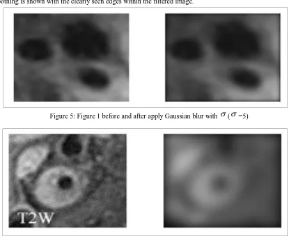
Figure 5: Figure 1 before and after apply Gaussian blur with
(
=5) [image:5.612.56.509.556.705.2]Figure 6: Figure 2 before and after apply Gaussian blur with
(
=5)Figure 5 and figure 6 illustrate the effects of more smoothening; figure-3 and figure-4 are obtained by use of constant
(
=2), and also figure-5 and figure-6 are obtained by use of constant
(
=5) and different from above value. It is noticed that increase in the value of
produces greater blurring of particular image. Generally, the effect of smoothing in the all the figures could be observed when compared right and left image of each figure.B. Mean filter
Figure 8: Figure 2 before and after applying average filter
Figure 7 shows the different image qualities before and after apply average filter. The noise is less and superficial, but the image has been `softened'.
Figure 8 shows the different image qualities before and after applying average filter. Salt and pepper noise are eliminated very effectively. However, noise pixel values are often very different from the surrounding values, and they tend to significantly distort the pixel average calculated by the mean filter.
[image:6.612.189.425.348.496.2]C. Histogram and histogram equalization : In the figure 9, the histogram of the original image shows farely high concentration of lower intensity pixels.
Figure 9: Pixel distribution of Figure 1
[image:6.612.172.418.548.706.2]The histogram of the original image (Figure 9) shows a large clustering of images on the far left - which corresponds to the overall low intensity of the image. After histogram equalization, the histogram density seems to have spread out over the intensity spectrum.
The effect on the image (Figure 10) is very obvious with a more expanded spread of intensities; the image appears much brighter as compared to the original. The equalization has not just brightened pixels; it has given a more even spread of intensities, so that the image has more brightness and contrast.
IV. CONCLUSION
Filters facilitate visual interpretation of images, and can also be used as an initial step to further image processing, such as segmentation. The use of filter also depends on the quality of raw data.
The filtration methods have many advantages and acquisitions to the image processing but there are also some disadvantages which can be eliminated by using specific functions and it also depends on applications. However, depending on application we can select any one or combination of methods to get the desired image processing output.
REFERENCES
[1] Bankman IN, Morcovescu S. Handbook of Medical Imaging. Processing and Analysis. Medical Physics. 2002 Jan 1;29(1):107.
[2] Davies, H. Magnetic Resonance Imaging (MRI), 2015. [online] EBME. Available at:
http://www.ebme.co.uk/articles/clinical-engineering/63-magnetic-resonance-imaging-mri.
[3] SAS, I. Image quality and artifacts in MRI. [online] IMAIOS, 2015. Available at:
http://www.imaios.com/en/e-Courses/e-MRI/Image-quality-and-artifacts/image-quality.
[4] Lagendijk RL, Biemond J. Basic Methods for Image Restoration and Identification-Chapter 14.
[5] Fabijańska, A. "Two-pass median filter for impulse noise removal." Automatyka/Akademia Górniczo-Hutnicza im. Stanisława Staszica w Krakowie 13 (2009): 807-820.
[6] Kathiravan, Srinivasan, and Jagannathan Kanakaraj. "A review on potential issues and challenges in MR imaging." The Scientific World Journal 2013 (2013).
[7] Bellon EM, Haacke EM, Coleman PE, Sacco DC, Steiger DA, Gangarosa RE. MR artifacts: a review. American Journal of Roentgenology. 1986 Dec
1;147(6):1271-81
[8] Jabbar R. A Study of Preprocessing and Segmentation Techniques on Cardiac Medical Images. International Journal of Engineering. 2014 Apr;3(4).
[9] Anitha, G., and Dr M. Hemalatha. "Intrusion prevention and Message Authentication Protocol (IMAP) using Region Based Certificate Revocation List Method in Vehicular Ad hoc Networks." International Journal of Engineering and Technology 6 (2014).
[10] Hsiao, Pei-Yung, Shin-Shian Chou, and Feng-Cheng Huang. "Generic 2-d gaussian smoothing filter for noisy image processing." TENCON 2007-2007 IEEE Region 10 Conference. IEEE, 2007.
[11] Fisher R, Perkins S, Walker A, Wolfart E. Gaussian smoothing. Hypermedia Image Processing Reference. 2003.
[12] Hsiao, Pei-Yung, Shin-Shian Chou, and Feng-Cheng Huang. "Generic 2-d gaussian smoothing filter for noisy image processing." TENCON 2007-2007 IEEE Region 10 Conference. IEEE, 2007.
[13] Deepa, P., and M. Suganthi. "Performance evaluation of various denoising filters for medical image." International Journal of Computer Science and Information Technologies 5.3 (2014): 4205-4209.
[14] Adam MY, Saeed MM, Al Samani A. Medical Image Enhancement Application Using Histogram Equalization in Computational Libraries.
[15] Bagade SS, Shandilya VK. Use of histogram equalization in image processing for image enhancement. International Journal of Software Engineering Research