SQUID: transcriptomic structural variation detection from RNA seq

M E T H O D

Open Access

SQUID: transcriptomic structural variation

detection from RNA-seq

Cong Ma, Mingfu Shao and Carl Kingsford

Abstract

Transcripts are frequently modified by structural variations, which lead to fused transcripts of either multiple genes, known as a fusion gene, or a gene and a previously non-transcribed sequence. Detecting these modifications, called transcriptomic structural variations (TSVs), especially in cancer tumor sequencing, is an important and challenging computational problem. We introduce SQUID, a novel algorithm to predict both fusion-gene and non-fusion-gene TSVs accurately from RNA-seq alignments. SQUID unifies both concordant and discordant read alignments into one model and doubles the precision on simulation data compared to other approaches. Using SQUID, we identify novel non-fusion-gene TSVs on TCGA samples.

Keywords: Transcriptomic structural variation, RNA-seq, TCGA

Background

Large-scale transcriptome sequence changes are known to be associated with cancer [1,2]. Those changes are usually a consequence of genomic structural variation (SV). By pulling different genomic regions together or separating one region into pieces, structural variants can potentially cause severe alteration to transcribed or translated prod-ucts. Transcriptome changes induced by genomic SVs, called transcriptomic structural variants (TSVs), can have a particularly large impact on disease genesis and pro-gression. In some cases, TSVs bring regions from one gene next to regions of another, causing exons from both genes to be transcribed into a single transcript (known as a fusion gene). Domains of the corresponding RNA or proteins can be fused, inducing new functions or causing loss of function, or the transcription or translation lev-els can be altered, leading to disease states. For example, BCR-ABL1is a well-known fusion oncogene for chronic myeloid leukemia [3], and the TMPRSS2-ERG fusion product leads to over-expression ofERGand helps trig-gers prostate cancer [4]. These fusion events are used as biomarkers for early diagnosis or treatment targets [5]. In other cases, TSVs can affect genes by causing a previously non-transcribed region to be incorporated into a gene,

*Correspondence:[email protected]

Computational Biology Department, School of Computer Science, Carnegie Mellon University, 5000 Forbes Ave., Pittsburgh, PA, USA

causing disruption to the function of the altered gene. There have been fewer studies on these TSVs between transcribed and non-transcribed regions, but their ability to alter downstream RNA and protein structure is likely to lead to similar results as fusion-gene TSVs.

Genomic SVs are typically detected from whole-genome sequencing (WGS) data by identifying reads and read pairs that are incompatible with a reference genome (e.g., [6–11]). However, WGS data are not completely suitable for inferring TSVs since they neither inform which region is transcribed nor reveal how the transcribed sequence will change if SVs alter a splicing site or the stop codon. In addition, WGS data are scarcer and more expensive to obtain than RNA-seq measurements [12], which target transcribed regions directly. RNA-seq is relatively inex-pensive, high-throughput, and widely available in many existing and growing data repositories. For example, The Cancer Genome Atlas (TCGA,https://cancergenome.nih. gov) contains RNA-seq measurements from thousands of tumor samples across various cancer types, but 80% of tumor samples in TCGA have RNA-seq data but no WGS data (Additional file1: Figure S1). While methods exist to detect fusion genes from RNA-seq measure-ments (e.g., [13–21]), fusion genes are only a subset of TSVs, and existing fusion-gene detection methods rely heavily on current gene annotations and are gener-ally not able or at least not optimized to predict non-fusion-gene TSV events. De novo transcript assembly

(e.g., [22–25]) followed by transcript-to-genome align-ment (e.g., [26–28]) is used in some fusion-gene detection methods. These approaches rely on annotation-based fil-tering steps to achieve high accuracy. Although it is pos-sible to extend these approaches to non-fusion-gene TSV detection, the lack of annotation information for non-transcribing regions makes these approaches less suitable for finding non-fusion-gene TSVs. This motivates the need for a method to detect both types of TSVs directly from RNA-seq data.

We present SQUID, the first computational tool that is designed to predict both types of TSVs comprehensively from RNA-seq data. SQUID divides the reference genome into segments and builds a genome segment graph (GSG) from both concordant and discordant RNA-seq read alignments. Using an efficient, novel integer linear pro-gram (ILP), SQUID rearranges the segments in the GSG so that as many read alignments as possible are concor-dant with the rearranged sequence. TSVs are represented by pairs of breakpoints realized by the rearrangement. In this way, it can detect both fusion-gene events and TSVs incorporating previously non-transcribed regions in tran-scripts. Discordant reads that cannot be made concordant through the optimal rearrangement given by the ILP are discarded as false positive discordant reads, likely due to misalignments. By building a consistent model of the entire rearranged genome and maximizing the number of overall concordant read alignments, SQUID drastically reduces the number of spurious TSVs reported compared with other methods.

SQUID is highly accurate. It is usually>20% more accu-rate than applying WGS-based SV detection methods to RNA-seq data directly. It is similarly more accurate than the pipeline that uses de novo transcript assembly and transcript-to-genome alignment to detect TSVs. We also show that SQUID is able to detect more TSVs involv-ing non-transcribed regions than any existinvolv-ing fusion-gene detection method.

We use SQUID to detect TSVs within 401 TCGA tumor samples of four cancer types (99–101 samples each of breast invasive carcinoma [29], bladder urothelial car-cinoma [30], lung adenocarcinoma [31], and prostate adenocarcinoma [32]). SQUID’s predictions suggest that breast invasive carcinoma has a larger variance in terms of number of TSVs/non-fusion-gene TSVs per sample than other cancer types. We also characterize the dif-ferences between fusion-gene TSVs and non-fusion-gene TSVs. Observed non-fusion-gene TSVs, for example, are more likely to be intra-chromosomal events. We show that similar breakpoints can occur in multiple samples, and among those that do repeatedly occur, their breakpoint partners are also often conserved. Finally, we identify several novel non-fusion-gene TSVs that affect known tumor suppressor genes (TSGs), which may result in loss

of function of corresponding proteins and play a role in tumorigenesis.

Results

A novel algorithm for detecting TSVs from RNA-seq

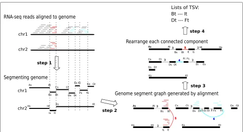
SQUID predicts TSVs from RNA-seq alignments to the genome (Fig.1provides an overview). To do this, it seeks to rearrange the reference genome to make as many of the observed alignments consistent with the rearranged genome as possible. Formally, SQUID constructs a graph from the alignments where the nodes represent bound-aries of genome segments and the edges represent adja-cencies implied by the alignments. These edges represent both concordant and discordant alignments, where con-cordant alignments are those consistent with the reference genome and discordant alignments are those that are not. SQUID then uses ILP to order and orient the vertices of the graph to make as many edges consistent as possible. Adjacencies that are present in this rearranged genome but not present in the original reference are proposed as predicted TSVs. The identification of concordant and discordant alignments, construction of the genome seg-ments, creation of the graph, and the reordering objective function are described in the “Methods” section.

SQUID is accurate on simulated data

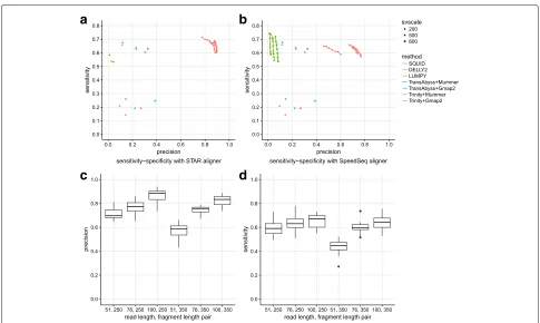
Overall, SQUID’s predictions of TSVs are far more pre-cise than other approaches at similar sensitivity on sim-ulated data. SQUID achieves 60% to 80% precision and about 50% sensitivity on simulation data (Fig. 2a, b). SQUID’s precision is>20% higher than several de novo transcriptome assembly and transcript-to-genome align-ment pipelines (for details see Additional file1: Additional Text), and the precision of WGS-based SV detection methods on RNA-seq data is even lower. The sensitivity of SQUID is similar to de novo assembly with MUMmer3 [26], but a little lower than DELLY2 [6] and LUMPY [7] with the SpeedSeq [33] aligner. The overall sensitivity is not as high as the precision, which is probably because there are not enough supporting reads aligned correctly to some TSV breakpoints. That assembly and WGS-based SV detection methods achieve similar sensitivity corrob-orates the hypothesis that the data limit the achievable sensitivity.

Fig. 1Overview of the SQUID algorithm. Based on the alignments of RNA-seq reads to the reference genome, SQUID partitions the genome into segments (step 1), connects the endpoints of the segments to indicate the actual adjacency in transcript (step 2), and finally reorders the endpoints along the most reliable path (step 3). Thick black lines are genome sequences or segments. Grey, red, and cyan short lines are read alignments, where grey represents concordant alignment, and red and cyan represent discordant alignments of different candidate TSVs. Vertical dashed lines are the separation boundaries between genome segments, and the boundaries are derived based on read alignments. The heads of genome segments are denoted by As, Bs, etc., and the tails are denoted by At, Bt, etc. Step 2: Each read alignment generates one edge between segment endpoints. An edge is added in the following way. When traversing the genome segments along the edge to generate a new sequence, the read can be aligned concordantly onto the new sequence. Multi-edges are collapsed into one weighted edge, where the weight is the number of reads supporting that edge. Red and cyan edges correspond to different candidate TSVs. Step 3: Genome segments are reordered and reoriented to maximize the total number of concordant alignments (concordant edge weights) with respect to the new sequence. Step 4: Discordant edges that are concordant after rearrangement are output as TSVs (in this case, both red edges and cyan edges are output). chr chromosome, TSV transcriptomic structural variant

which up-weights initially discordant reads to com-pensate for heterogeneous mixtures, does not affect precision or sensitivity in simulation data because sim-ulated reads are homogeneous, and there is no need to adjust for the normal/tumor cell ratio (Additional file1: Figure S2e, f ).

We also test the robustness of SQUID against different RNA-seq experimental settings. Specifically, we simulate RNA-seq data with read lengths of 51, 76 and 100 bp combined with fragment lengths of 250 bp and 350 bp (Fig. 2c, d). For the full table showing the accuracy of SQUID and other methods, see Additional file 2. Each experimental setting has four replicates. With increased read length, SQUID in general performs better in both precision and sensitivity (although there are a few excep-tions where the randomness of the simulation shad-ows the benefit from the longer read length). However, with increased fragment length, SQUID performs slightly worse. In this case, there are fewer reads aligned at the exact breakpoint, possibly due to an increase in split-alignment difficulty for aligners. A short read length

(51 bp) with long fragment length (350 bp) leads to the worst precision and sensitivity.

a

b

c

d

Fig. 2Performance of SQUID and other methods on simulation data.a,bDifferent numbers of SVs (200, 500, and 800 SVs) are simulated in each dataset. Each simulated read is aligned with the aligners (a) STAR and (b) SpeedSeq. If the method allows for user-defined minimum read support for prediction, we vary the threshold from 3 to 9, and plot a sensitivity–precision curve (SQUID and LUMPY), otherwise it is shown as a single point. c,dPerformance of SQUID under different RNA-seq experimental parameter combinations (read lengths of 51, 76, and 100 bp combined with fragment lengths of 250 and 350). A longer read length increases both the precision and sensitivity of SQUID. A longer fragment length slightly decreases SQUID’s performance. A short read length with a long fragment length leads to the worst precision and sensitivity. SV structural variant

SQUID’s effectiveness is likely due to its unified model for both concordant reads and discordant reads. Cover-age in RNA-seq alignment is generally proportional to the expression level of the transcript, and using one read count threshold for TSV evidence is not appropriate. Instead, the ILP in SQUID puts concordant and discor-dant alignments into competition and selects the winner as the most reliable TSV.

SQUID is able to detect non-fusion-gene TSVs for two previously studied cell lines

Fusion-gene events are a strict subset of TSVs where the two breakpoints are each within a gene region and the fused sequence corresponds to the sense strand of both genes. Fusion genes, thus, exclude TSV events where a gene region is fused with an intergenic region or an anti-sense strand of another gene. Nevertheless, fusion genes have been implicated in playing a role in cancer.

To probe SQUID’s ability to detect both fusion-gene and non-fusion-gene TSVs from real data, we use two cell lines, HCC1954 and HCC1395, both of which are tumor epithelial cells derived from breast. Previous stud-ies have experimentally validated the predicted SVs and

fusion-gene events for these two cell lines. Specifically, we compile results from [34–38] for HCC1954 and results from [13, 35] for HCC1395. After removing short dele-tions and overlapping SVs from different studies, we have 326 validated SVs for the HCC1954 cell line, of which 245 have at least one breakpoint outside a gene region, and the rest (81) have both breakpoints within a gene region. In addition, we have 256 validated true SVs for the HCC1395 cell line, of which 94 have at least one breakpoint outside a gene region, while the rest (162) have both breakpoints within a gene. For a predicted SV to be a true positive, both predicted breakpoints should be within a window of 30 kb of true breakpoints and the predicted orientation should agree with the true orientation. We use a relatively large window, since the true breakpoints can be located within an intron or other non-transcribed region, while the observed breakpoint from RNA-seq reads will be at a nearby coding or expressed region.

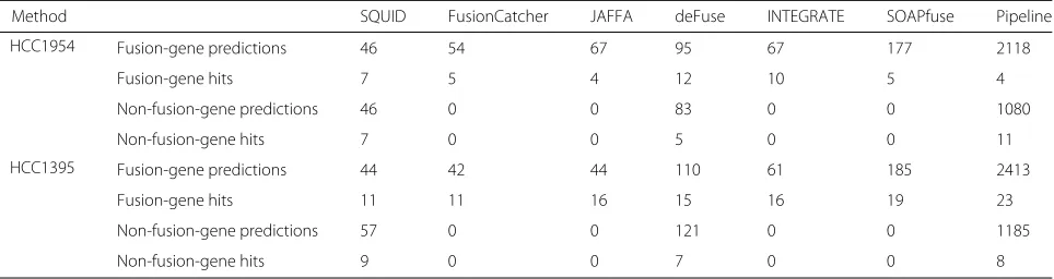
experiments, the sample from which RNA-seq was col-lected may be different from those used for experimental validation. We align reads to the reference genome using STAR. We compare the result with the top fusion-gene detection tools evaluated in [42] and newer software not evaluated by [42], specifically, SOAPfuse [20], deFuse [14], FusionCatcher [16], JAFFA [15], and INTEGRATE [15]. In addition, we compare to the same pipeline of de novo transcriptome assembly and transcript-to-genome align-ment as in the previous section (also see Additional file1: Additional Text). Trans-ABySS [22] is chosen for the de novo transcriptome assembly and MUMmer3 [26] is chosen for the transcript-to-genome alignment, because this combination performed the best with simulation data. Table1summarizes the total number of predicted TSVs, and the number of TSVs corresponding to pre-viously validated TSVs (hits). For the full list of TSV predictions by SQUID for the two cell lines, refer to Additional files3and4.

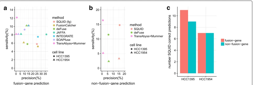
When restricted to fusion-gene events, SQUID achieves similar precision and sensitivity compared to fusion-gene detection tools (Fig. 3a). These methods have different rankings for the two cell lines. There is no uniformly best method for fusion-gene TSV predictions for both cell lines. SQUID has one of the highest precision val-ues and the second highest sensitivity for the HCC1954 cell line and ranks in the middle for the HCC1395 cell line. For both cell lines, the pipeline of de novo transcrip-tome assembly and transcript-to-genome alignment has very low precision, which suggests that without filtering steps, assembly-based methods are not able to distinguish between noise and true TSVs.

It is even harder to predict non-fusion-gene TSVs accu-rately, since current annotations cannot be used to limit the search space for potential read alignments or TSV events. Only SQUID, deFuse, and the pipeline of de novo transcriptome assembly and transcript-to-genome align-ment are able to detect non-fusion-gene events. SQUID has both a higher precision and a higher sensitivity com-pared to deFuse (Fig. 3b). The assembly pipeline has a higher sensitivity but very low precision, which again

indicates that this pipeline outputs non-fusion-gene TSV signals without distinguishing them from noise. A con-siderable proportion of validated TSVs are non-fusion-gene TSVs. Correctly predicted non-fusion-non-fusion-gene TSVs make up almost half of all correct predictions of SQUID (Fig.3c).

We test the robustness of SQUID with respect to dif-ferent parameter values on the two cell lines (Additional file3: Figure S3). We find the same trend regarding the segment degree threshold and the edge weight old as with simulated data. The segment degree thresh-old does not affect either precision or sensitivity much, and the edge weight threshold determines the precision– sensitivity tradeoff. The discordant edge weight coeffi-cient does not change the sensitivity on the HCC1954 cell line, possibly indicating that the sequencing data is relatively homogeneous. As this parameter increases, pre-cision for the HCC1954 cell line slightly decreases because more TSVs are predicted. In contrast, an increase of the discordant edge weight coefficient increases both the precision and sensitivity of the HCC1395 cell line. This implies that for some transcripts, normal reads dominate tumor reads, and increasing this parameter allows us to identify those TSVs.

The sensitivity for both cell lines of all tested methods is relatively low. One explanation for this is the difference between the source of the data used for prediction and val-idation. In the ground truth, some SVs were first identified using WGS data or BAC end sequencing and then vali-dated experimentally. Not all genes are expressed in the RNA-seq data used here, and lowly expressed genes may not generate reads spanning SV breakpoints due to read sampling randomness. To quantify the feasibility of each SV being detected, we count the number of supporting chimeric reads in RNA-seq alignments. The proportion of ground-truth fusion-gene TSVs with supporting reads is very low for both cell lines: 26.5% for HCC1954 (13 out of 49) and 27.1% for HCC1395 (47 out of 173). The max-imum sensitivity of fusion-gene TSV prediction is limited by these numbers, which explains the relatively low sensi-tivity we observed. For non-fusion-gene TSVs, only 13.0%

Table 1Summary of TSV predictions for HCC1954 and HCC1395 cell lines

Method SQUID FusionCatcher JAFFA deFuse INTEGRATE SOAPfuse Pipeline

HCC1954 Fusion-gene predictions 46 54 67 95 67 177 2118

Fusion-gene hits 7 5 4 12 10 5 4

Non-fusion-gene predictions 46 0 0 83 0 0 1080

Non-fusion-gene hits 7 0 0 5 0 0 11

HCC1395 Fusion-gene predictions 44 42 44 110 61 185 2413

Fusion-gene hits 11 11 16 15 16 19 23

Non-fusion-gene predictions 57 0 0 121 0 0 1185

a

b

c

Fig. 3Performance of SQUID and fusion-gene detection methods on breast cancer cell lines HCC1954 and HCC1395. Predictions are evaluated for previously validated SVs and fusions.aFusion-gene prediction sensitivity–precision curve of different methods.bNon-fusion-gene prediction sensitivity–precision curve. Only SQUID, deFuse, and the pipeline of de novo transcriptome assembly and transcript-to-genome alignment are able to predict non-fusion-gene TSVs.cNumber of fusion-gene TSVs and non-fusion-gene TSVs correctly predicted by SQUID. Non-fusion-gene TSVs make up a considerable proportion of all TSVs. TSV transcriptomic structural variant

in HCC1954 (36 out of 277) and 21.7% in HCC1395 (13 out of 83) can possibly be identified.

We use WGS data for the corresponding cell lines to val-idate the novel TSVs predicted by SQUID (SRA accession numbers ERP000265 [43] for HCC1954 and SRR892417 [44] and SRR892296 [45] for HCC1395). For each TSV prediction, we extract a 25-kb sequence around both breakpoints and concatenate them according to the pre-dicted TSV orientation. We then map the WGS reads against these junction sequences using SpeedSeq [33]. If a paired-end WGS read can be mapped only concordantly to a junction sequence but not to the reference genome, that paired-end read is marked as supporting the TSV. If at least three WGS reads support a TSV, the TSV is considered as validated. With this approach, we are able to validate 40 more TSV predictions for the HCC1395 cell line and 18 more TSV predictions for the HCC1954 cell line. In total, the percentage of predicted TSVs that can be validated either by previous studies or by WGS data is 57.7% for the HCC1395 cell line and 35.2% for the HCC1954 cell line. The WGS validation rate of the HCC1954 cell line is much lower than for the HCC1395 cell line, which can be explained by the relatively low read depth. The read depth for HCC1954 WGS data is 7.6× and that for HCC1395 WGS data is 22.7×.

Characterizing TSVs on four types of TCGA cancer samples

To compare the distributions and characteristics of TSVs among cancer types and between TSV types, we applied SQUID on arbitrarily selected 99 to 101 tumor sam-ples from TCGA for each of four cancer types: breast invasive carcinoma (BRCA), bladder urothelial carcinoma (BLCA), lung adenocarcinoma (LUAD), and prostate ade-nocarcinoma (PRAD). TCGA aliquot barcodes of the

corresponding samples are listed in Additional file5. For data processing details, see Additional file 1: Additional Text. The running time of SQUID is less than 3 hours for the majority of the RNA-seq data we selected, and the maximum memory usage is around 4 or 8 GB (Additional file1: Figure S4).

To estimate the accuracy of SQUID’s prediction for selected TCGA samples, we use WGS data for the same patients to validate TSV junctions. There are 72 WGS experiments available for the 400 samples (20 BLCA, 10 BRCA, 31 LUAD, and 11 PRAD). We use the same approach with WGS to validate SQUID predictions as in the previous section. SQUID’s overall validation rate is 88.21%, which indicates that SQUID is quite accurate and reliable on TCGA data.

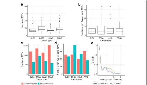
We find that most samples have∼18–23 TSVs, includ-ing ∼3–4 non-fusion-gene TSVs among all four cancer types (Fig. 4a, b). For BRCA, the tail of the distribu-tion of TSV counts is larger, and more samples contain a larger number of TSVs. The same trend is observed when restricted to non-fusion-gene TSVs.

a

b

c

d

e

Fig. 4 a,bNumber of TSVs and non-fusion-gene TSVs in each sample in different cancer types. BRCA has slightly more samples with a larger number of (non-fusion-gene) TSVs. Thus, it has a longer tail on they-axis.c,dNumber of inter-chromosomal and intra-chromosomal TSVs within all TSVs and within non-fusion-gene TSVs. Non-fusion-gene TSVs contain more intra-chromosomal events than fusion-gene TSVs. (e) For breakpoints occurring more than 3 times in the same cancer type, the distribution of the entropy of its TSV partner. The lower the entropy, the more likely it is that the breakpoint has a fixed partner. The peak near 0 indicates a large portion of breakpoints are likely to be rejoined with the same partner in the TSV. However, there are still some breakpoints that have multiple rejoined partners. BLCA bladder urothelial carcinoma, BRCA breast invasive carcinoma, LUAD lung adenocarcinoma, PRAD prostate adenocarcinoma, TSV transcriptomic structural variant

percentage of intra-chromosomal TSVs within non-fusion-gene TSVs is higher than that within all TSVs.

For a large proportion of breakpoints occurring multi-ple times within a cancer type, their partner in the TSV is likely to be fixed and to reoccur every time that break-point is used. To quantify this, for each breakbreak-point that occurred≥3 times, we compute the entropy of its partner promiscuity. Specifically, we derive a discrete empirical probability distribution of partners for each breakpoint and compute the entropy of this distribution. This mea-sure, thus, represents the uncertainty of the partner given one breakpoint, with higher entropy corresponding to a less conserved partnering pattern. In Fig.4e, we see that there is a high peak near 0 for all cancer types, which indi-cates that for a large proportion of recurring breakpoints, we are certain about its rejoined partner once we know the breakpoint. However, there are also promiscuous break-points with entropy larger than 0.5.

Tumor suppressor genes can undergo TSV and generate altered transcripts

TSGs protect cells from becoming cancer cells. Usually their functions involve inhibiting cell cycle, facilitating

apoptosis, and so on [46]. Mutations in TSGs may lead to loss of function of the corresponding proteins and benefit tumor growth. For example, a homozygous loss-of-function mutation in p53 is found in about half of cancer samples across various cancer types [47]. TSVs are likely to cause loss of function of TSGs as well. Indeed, we observe several TSGs that are affected by TSVs, both of the fusion-gene type and the non-fusion-gene type.

a

b

c

d

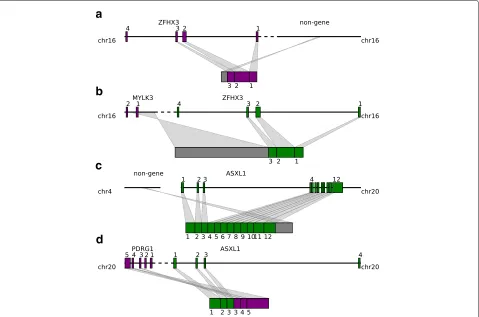
Fig. 5Tumor suppressor genes are affected by both fusion-gene and non-fusion-gene TSVs and generate transcripts with various features.aZFHX3

is fused with an intergenic region after exon 3. The transcript stops at the inserted region, losing the rest of the exons.bZFHX3is fused with a part of theMYLK3anti-sense strand after exon 3. Codon and splicing signals are not preserved on anti-sense strands, thus, anMYLK3anti-sense insertion acts like an intergenic region insertion and causes transcription to stop before reaching the rest of theZFHX3exons.cASXL1is fused with an intergenic region in the middle of exon 12. The resulting transcript contains a truncatedASXL1exon 12 and intergenic sequence.dThe first three exons of theASXL1gene are joined with the last three exons ofPDRG1, resulting in a fused transcript containing six complete exons from both

ASXL1andPDRG1. chr chromosome, TSV transcriptomic structural variant

not preserved on the anti-sense strand, the transcribed insertion region does not correspond to known exons of theMYLK3gene, but covers the range of the first exon of MYLK3and extends to the first intron and 5 intergenic region. Transcription stops within the inserted region, and causes theZFHX3transcript to lose exons after exon 3, which resembles the fusion with the intergenic region in the BLCA sample.

Another example is given by theASXL1gene, which is essential for activating CDKN2Bto inhibit tumorigene-sis [50]. We observe two distinct TSVs related toASXL1 from BLCA and BRCA samples. The first TSV merges the first 11 exons and half of exon 12 ofASXL1with an intergenic region on chromosome 4 (Fig.5c, Additional file1: Figure S7). Transcription stops at the inserted inter-genic region, leaving the rest of exon 12 untranscribed. The breakpoint within ASXL1 is before the 3 untrans-lated region, so the downstream protein sequence from exon 12 will be affected. The other TSV involvingASXL1

is a typical fusion-gene TSV where the first three exons of ASXL1 are fused with the last three exons from the PDRG1gene (Fig.5d, Additional file1: Figure S8). Protein domains afterASXL1exon 4 and beforePDRG1exon 2 are lost in the fused transcript.

These non-fusion-gene examples are novel predicted TSV events, which are not typically detectable via tra-ditional fusion-gene detection methods using RNA-seq data. They suggest that non-fusion-gene events can also be involved in tumorigenesis by disrupting TSGs.

Discussion

and by rearranging genome segments to maximize the number of concordant reads, SQUID generates a set of compatible TSVs that are most reliable in terms of the numbers of reads supporting them. Instead of a universal read support threshold, the objective function in SQUID naturally balances reads supporting and not supporting a candidate TSV. This design is efficient in filtering out sequencing and alignment noise in RNA-seq, especially in the annotation-free context of predicting non-fusion-gene TSV events.

By applying SQUID to TCGA RNA-seq data, we are able to detect TSVs in cancer samples, especially non-fusion-gene TSVs. We identify novel non-non-fusion-gene TSVs involving the known TSGs ZFHX3 and ASXL1. Both fusion-gene and non-fusion-gene events detected in TCGA samples are computational predictions and need further experimental validation.

Other important uses and implications for general TSVs have yet to be explored and represent possible direc-tions for future work. TSVs will impact the accuracy of transcriptome assembly and expression quantification, and methodological advances are needed to correct those downstream analyses for the effect of TSVs. For exam-ple, current reference-based transcriptome assemblers are not able to assemble from different chromosomes for inter-chromosomal TSVs. In addition, expression levels of TSV-affected transcripts cannot be quantified if they are not present in the transcript database. Incorporating TSVs into transcriptome assembly and expression quan-tification can potentially improve their accuracy. SQUID’s ability to provide a new genome sequence that is as con-sistent as possible with the observed reads will facilitate its use as a preprocessing step for transcriptome assem-bly and expression quantification, though optimizing this pipeline remains a task for future work.

Several natural directions exist for extending SQUID. First, SQUID is not able to predict small deletions. Instead, it treats small deletions the same as introns. This is to some extent a limitation of using RNA-seq data. Introns and deletions are difficult to distinguish, as both result in concordant split reads or stretched mate pairs. Using gene annotations could somewhat address this problem. Second, when the RNA-seq reads are derived from a highly heterogeneous sample, SQUID is likely not able to predict all TSVs in the same region if they conflict, since it seeks a single consistent genome model. Instead, SQUID will pick only the dominating one that is compat-ible with other predicted TSVs. One approach to handle this would be to re-run SQUID iteratively, removing reads that are explained at each step. Again, this represents an attractive avenue for future work.

SQUID is open source and available at http:// www.github.com/Kingsford-Group/squidand the scripts to replicate the computational experiments described

here are available at http://www.github.com/Kingsford-Group/squidtest.

Conclusion

We developed SQUID, the first algorithm to detect TSVs accurately and comprehensively that targets both tradi-tional fusion-gene detection and the much broader class of general TSVs. SQUID exhibits higher precision at sim-ilar sensitivities compared with WGS-based SV detection methods and pipelines of de novo transcriptome assembly and transcript-to-genome alignment. In addition, it can detect non-fusion-gene TSVs with similarly high accuracy. We use SQUID to predict TSVs in TCGA tumor sam-ples. From our prediction, BRCA has a slightly flatter distribution of the number of per-sample TSVs than the other cancer types studied. We observe that non-fusion-gene TSVs are more likely to be intra-chromosomal events than fusion-gene TSVs. This is likely due to the differ-ent sequence composition features in gene vs. non-gene regions. PRAD also stands out because it has the largest percentage of inter-chromosomal TSVs. Overall, these findings continue to suggest that different cancer types have different preferred patterns of TSVs, although the question remains whether these differences will hold up as more samples are analyzed and whether the different patterns are causal, correlated, or mostly due to non-functional randomness. These findings await experimen-tal validation.

As shown by predictions from SQUID, TSGs are involved in non-fusion-gene TSVs. In these cases, tran-scription usually stops within the inserted region of the non-fusion-gene TSVs, which causes the TSG transcript to lose some of its exons, and possibly leads to down-stream loss of function. The large-scale variations of TSGs suggest that non-fusion-gene TSVs can potentially affect cancer genesis and progression, and needs to be studied more carefully.

Methods

The computational problem: rearrangement of genome segments

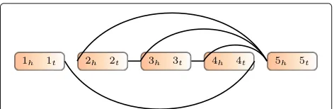
We formulate the TSV detection problem as the optimiza-tion problem of rearranging genome segments to max-imize the number of observed reads that are consistent (termed concordant) with the rearranged genome. This approach requires defining the genome segments that can be independently rearranged. It also requires defin-ing which reads are consistent with a particular arrange-ment of the segarrange-ments. We will encode both of these (segments and read consistency) within a GSG. Fig.6is an example.

Fig. 6Example of a genome segment graph. Boxes are genome segments, each of which has two ends with subscriptshandt. The color gradient indicates the orientation from head to tail. Edges connect the ends of genome segments

genome. sh represents its head and st its tail in reference genome coordinates. In practice, segments will be derived from read locations.

Definition 2(Genome Segment Graph (GSG))A GSG G = (V,E,w) is an undirected weighted graph, where V contains both endpoints of each segment in a set of segments S, i.e., V = {sh: s∈S} ∪ {st:s∈S}. Thus, each vertex in the GSG represents a location in the genome. An edge (u,v) ∈ E indicates that there is evidence that the location u is adjacent to location v. The weight function w:E −→R+represents the reliability of an edge. Gener-ally speaking, the weight is the number of read alignments supporting the edge, but we use a multiplier to calculate edge weights, which is discussed below. In practice, E and w will be derived from split-aligned and paired-end reads.

Defining vertices by endpoints of segments is required to avoid ambiguity. Knowing only that segmentiis con-nected with segment j is not enough to recover the sequence, since different relative positions ofiandjspell out different sequences. Instead, for example, an edge

(it,jh) indicates that the tail of segment i is connected to the head of segment j, and this specifies a unique desired local sequence with the only other possibility being the reverse complement (i.e., it could be that the true sequence is i · j or rev(j) · rev(i); here · indicates concatenation and rev(i) is the reverse complement of segmenti).

A GSG is similar to a breakpoint graph [51] but with critical differences. A breakpoint graph has edges repre-senting connections both in the reference genome and in the target genome. Edges in a GSG represent only the target genome, and they can be either concordant or dis-cordant. In addition, a GSG does not require that the degree of every vertex is 2, and thus, alternative splicing and erroneous edges can exist in a GSG.

Our goal is to reorder and reorient the segments in S so that as many edges in G are compatible with the rearranged genome as possible.

Definition 3(Permutation)A permutationπon a set of segments S projects a segment in S to a set of integers from 1 to|S|(the size of S), representing the indices of the segments in an ordering of S. In other words, each permutation π defines a new order of segments in S.

Definition 4 (Orientation Function)An orientation function f maps both ends of a segment to 0 or 1:

f :{sh:s∈S} ∪ {st:s∈S} −→ {0, 1},

subject to f(s_h)+f(st) =1for all s=(sh,st) ∈S. An ori-entation function specifies the oriori-entations of all segments in S. Specifically, f(sh)=1means shgoes first and stnext, corresponding to the forward strand of the segment, and f(st)=1corresponds to the reverse strand of the segment.

With a permutationπand an orientation functionf, the exact and unique sequence of a genome is determined. The reference genome also corresponds to a permutation and an orientation function, where the permutation is the identity permutation and the orientation function maps allshto 1 and allstto 0.

Definition 5 (Edge Compatibility)Given a set of seg-ments S, a GSG G = (V,E,w), a permutation π on S, and an orientation function f, an edge e = (ui,vj) ∈ E, where ui ∈ {uh,ut} and vj ∈ {vh,vt}, is compatible with permutationπand orientation f if and only if

1−f(vj)=1[π(v) < π(u)]=f(ui), (1)

where1[x]is an indicator function, which is 1 if x is true and 0 otherwise. Comparison between permuted elements is defined as comparing their index in permutation, that is,

π(v) < π(u)states that segment v is in front of segment u in rearrangementπ. We write e∼(π,f)if e is compatible withπand f.

The above two edge compatibility Eqs.1require that, for an edge to be compatible with the rearranged and reori-ented sequence determined byπandf, it needs to connect the right side of the segment in front to the left side of the segment following it. As we will see below, the edges of a GSG are derived from read alignments. An edge being compatible withπandf is essentially equivalent to stating that the corresponding read alignments are concordant with respect to the target genome determined byπandf. When(π,f)is clear, we refer to edges that are compati-ble as concordant edges and edges that are incompaticompati-ble as discordant edges.

With the above definitions, we formulate an optimiza-tion problem as follows:

Problem 1Input:A set of segments S and a GSG G =

Output: Permutationπ on S and orientation function f that maximizes:

max

π,f

e∈E

w(e)·1e∼(π,f). (2)

This objective function tries to find a rearrangement of genome segments(π,f)such that when aligning reads to the rearranged sequence, as many reads as possible will be aligned concordantly. This objective function includes both concordant alignments and discordant alignments and sets them in competition, which is effective in reduc-ing the number of false positives when tumor transcripts outnumber normal transcripts. There is the possibility that some rearranged tumor transcripts will be outnum-bered by normal counterparts. To be able to detect TSVs in this case, depending on the setting, we may weight discordant read alignments more than concordant read alignments. Specifically, for each discordant edge e, we multiply the weightw(e)by a constantαthat represents our estimate of the ratio of normal transcripts over tumor counterparts.

The final TSVs are modeled as pairs of breakpoints. Denote the permutation and orientation corresponding to an optimally rearranged genome as(π∗,f∗)and those that correspond to the reference genome as(π0,f0). An edgee can be predicted as a TSV ife∼(π∗,f∗)ande(π0,f0).

Integer linear programming formulation

We use ILP to compute an optimal solution(π∗,f∗) of Problem1. To do this, we introduce the following Boolean variables:

• xe=1if edgee∼(π∗,f∗)and 0 if not.

• zuv=1if segmentu is before v in the permutation

π∗_{and 0 otherwise.}

• yu=1iff∗(uh)=1for segmentu.

With this representation, the objective function can be rewritten as

max xe,yu,zuv

w(e)·xe. (3)

We add constraints to the ILP derived from edge com-patibility Eq.1. Without loss of generality, we first suppose segmentuis in front ofvin the reference genome, and edgeeconnectsutandvh (which is a tail–head connec-tion). Plugging inut, the first equation in (1) is equivalent to 1−1[π(u) > π(v)]=1−f(ut)and can be rewritten as

1[π(u) < π(v)]=f(uh) =yu. Note that1[π(u) < π(v)] has the same meaning as zuv; it leads to the constraint zuv = yu. Similarly, the second equation in (1) indicates zuv = yv. Therefore, xe can reach 1 only when yu = yv = zuv. This is equivalent to the inequalities (4) below. Analogously, we can write constraints for the other three

types of edge connections: tail–tail connections impose inequalities (5), head–head connections impose inequali-ties (6), and head–tail connections impose inequalities (7):

xe≤yu−yv+1, xe≤yv−yu+1, xe≤yu−zuv+1, xe≤zuv−yu+1,

(4)

xe≤yu−(1−yv)+1, xe≤(1−yv)−yu+1, xe≤yu−zuv+1, xe≤zuv−yu+1,

(5)

xe≤(1−yu)−yv+1, xe≤yv−(1−yu)+1, xe≤(1−yu)−zuv+1, xe≤zuv−(1−yu)+1,

(6)

xe≤(1−yu)−(1−yv)+1, xe≤(1−yv)−(1−yu)+1, xe≤(1−yu)−zuv+1, xe≤zuv−(1−yu)+1.

(7)

We also add constraints to enforce thatzuvforms a valid topological ordering. For each pair of nodesuandv, one must be in front of the other, that is zuv +zvu = 1. In addition, for each triple of nodes,u,v, andw, one must be at the beginning and one must be at the end. Therefore, we add 1≤zuv+zvw+zwu≤2.

Solving an ILP in theory takes exponential time, but in practice, solving the above ILP to rearrange genome segments is very efficient. The key is that we can solve for each connected component separately. Because the objective maximizes the sum of compatible edge weights, the best rearrangement of one connected component is independent of the rearrangement of another because, by definition, there are no edges between connected components.

Concordant and discordant alignments

a

d

e b

c

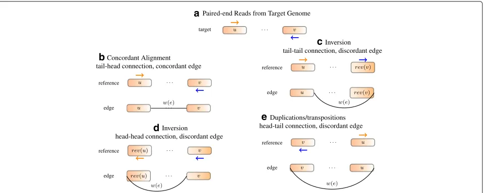
Fig. 7Constructing edges from alignment.aRead positions and orientations generated from the target genome.bIf the reference genome does not have rearrangements, the read should be concordantly aligned to the reference genome. An edge is added to connect the right end ofuto the left end ofv. Traversing the two segments along the edge reads outu_·v, which is the same as the reference.cBoth ends of the read align to the forward strand. An edge is added to connect the right end ofuto the right end of rev₍v₎. Traversing the segments along the edge reads out sequenceu_·rev₍rev₍v₎₎₌u_·v, which recovers the target sequence and the read can be concordantly aligned.dIf both ends align to the reverse strand, an edge is added to connect the left end of the front segment to the left end of the back segment.eIf two ends of a read point away from each other, an edge is added to connect the left end of the front segment to the right end of the back segment

requirements are invalid in RNA-seq alignments because alignments of reads can be separated by an intron with unknown length.

We define concordance criteria separately for split-alignment and paired-end split-alignment. If one end of a paired-end read is split into several parts and each part is aligned to a location, the end has split alignments. Denote the vector of the split alignments of an end as R= [A1,A2,. . .,Ar] (rdepends on the number of splits). Each alignmentR[i] = Ai has four components: a chro-mosome (Chr), an alignment starting position (Spos), an alignment ending position, and an orientation (Ori, with value either+or−). We require that the alignmentsAi are sorted by their position in the read. A split-aligned endR=[A1,A2,. . .,Ar] is concordant if all the following conditions hold:

Ai.Chr=Aj.Chr, ∀i,∀j, Ai.Ori=Aj.Ori, ∀i,∀j,

Ai.Spos<Aj.Spos, ifAi.Ori= +for alli<j, Ai.Spos>Aj.Spos, ifAi.Ori= −for alli<j.

(8)

If the end is not split, but continuously aligned, the alignment automatically satisfies Eq.8. Denote the align-ments ofR’s mate asM=[B1,B2,. . .,Bm]. An alignment of the paired-end read is concordant if the following conditions all hold:

Ai.Chr=Bj.Chr, ∀i,∀j, Ai.Ori=Bj.Ori, ∀i,∀j,

A1.Spos<Bm.Spos, ifA1.Ori= +, Am.Spos>B1.Spos, ifA1.Ori= −.

(9)

We require only that the leftmost split of the forward readRis in front of the leftmost split of the reverse read M, since the two ends in a read pair may overlap. For a paired-end read to be concordant, each end should satisfy split-read alignment concordance (8), and the pair should satisfy paired-end alignment concordance (9).

Splitting the genome into segmentsS

We use a set of breakpoints to partition the genome. The set of breakpoints contains two types of positions: (1) the start position and end position of each interval of overlap-ping discordant alignments and (2) an arbitrary position in each 0-coverage region.

segments in a GSG connected to their adjacent segments and thus, creating one big connected component, we pick the starting point of each 0-coverage region as a breakpoint. By adding those breakpoints, different genes will be in separate connected components unless some discordant reads support their connection. Overall, the size of each connected component is not very large. The number of nodes generated by each gene is approximately the number of exons located in them and these gene subgraphs are connected only when there is a potential TSV between them.

Defining edges and filtering out obvious false positives

In a GSG, an edge is added between two vertices when there are reads supporting the connection. For each read spanning different segments, we build an edge such that when traversing the segments along the edge, the read is concordant with the new sequence [Eqs. (8) and (9)]. Examples of deriving an edge from a read alignment are given in Fig.7. In this way, the concordance of an align-ment and the compatibility of an edge with respect to a genome sequence are equivalent.

The weight of a concordant edge is the number of read alignments supporting the connection, while the weight of a discordant edge is the number of supporting alignments multiplied by the discordant edge weight coefficient α. The discordant edge weight coefficientα represents the normal/tumor cell ratio (for a complete table of SQUID parameters, see Additional file1: Table S1). If normal tran-scripts dominate tumor trantran-scripts,αenlarges the discor-dant edge weights and helps to satisfy the discordiscor-dant edges in the rearrangement of the ILP.

We filter out obvious false positive edges to reduce both the ILP computation time and the mistakes after the ILP. Edges with very low read support are likely to be a result of alignment error, therefore, we filter out edges with a weight lower than a thresholdθ. Segments with too many connections to other regions are likely to have low map-pability, so we also filter out segments connecting to more thanγ other segments. The parametersα, θ, andγ are the most important user-defined parameters in SQUID (Additional file1: Table S1, Figures S2 and S3). An inter-leaving structure of exons from different regions (different genes) seems more likely to be a result of sequencing or alignment error rather than an SV. Thus, we filter out the interleaving edges between two such groups of segments.

Identifying TSV breakpoint locations

Edges that are discordant in the reference genome indicate potential rearrangements in transcripts. Among those edges, some are compatible with the permutation and orientation from ILP. These edges are taken to be the pre-dicted TSVs. For each edge that is discordant initially but compatible with the optimal rearrangement found by ILP,

we examine the discordant read alignments to determine the exact breakpoint within related segments. Specifi-cally, for each end of a discordant alignment, if there are two other read alignments that start or end in the same position and support the same edge, then the end of the discordant alignment is predicted to be the exact TSV breakpoint. Otherwise, the boundary of the corresponding segment will be output as the exact TSV breakpoint.

Simulation methodology

Simulations with randomly added SVs and simu-lated RNA-seq reads were used to evaluate SQUID’s performance in situations with a known correct answer. RSVsim [52] was used to simulate SVs in the human genome (Ensembl 87 or hg38) [53]. We use the five longest chromosomes for simulation (chromosome 1 to chromosome 5). RSVsim introduces five different types of SVs: deletion, inversion, insertion, duplication, and inter-chromosomal translocation. To vary the complexity of the resulting inference problem, we simulated genomes with 200 SVs of each type, 500 SVs of each type, and 800 SVs of each type. We generated four replicates for each level of SV complexity (200, 500, and 800). For inter-chromosomal translocations, we simulate only two events because only five chromosomes were used.

In the simulated genome with SVs, the original gene annotations are not applicable, and we cannot simulate gene expression from the rearranged genome. Therefore, for testing, we interchange the roles of the reference (hg38) and the rearranged genome, and use the new genome as the reference genome for alignment, and hg38 with the original annotated gene positions as the target genome for sequencing. Flux Simulator [54] was used to simulate RNA-seq reads from the hg38 genome using Ensembl annotation version 87 [55].

After simulating SVs in the genome, we need to trans-form the SVs into a set of TSVs, because not all SVs affect the transcriptome, and thus, not all SVs can be detected by RNA-seq. To derive a list of TSVs, we compare the positions of simulated SVs with the gene annotation. If a gene is affected by an SV, some adjacent nucleotides in the corresponding transcript may be in a far part of the RSVsim-generated genome. The adjacent nucleotides may be consecutive nucleotides inside an exon if the break-point breaks the exon, or the endbreak-points of two adjacent exons if the breakpoint hits the intron. So for each SV that hits a gene, we find the pair of nucleotides that are adja-cent in the transcript and separated by the breakpoints, and convert them into the coordinates of the RSVsim-generated genome, thus, deriving the TSV.

whether existing WGS-based SV detection methods can be directly applied to RNA-seq data. For the de novo tran-scriptome assembly and transcript-to-genome alignment pipeline, we use all combinations of the existing software Trinity [23], Trans-ABySS [22], GMAP [27], and MUM-mer3 [26]. For WGS-based SV detection methods, we test LUMPY [7] and DELLY2 [6]. We test both STAR [56] and SpeedSeq [33] (which is based on BWA-MEM [57]) to align RNA-seq reads to the genome. LUMPY is compati-ble only with the output of SpeedSeq, so we do not test it with STAR alignments.

Additional files

Additional file 1: Additional Text,Table S1with descriptions,Figures S1–S8with descriptions. (PDF 2979 kb)

Additional file 2: Precision and sensitivity table for simulated data with different read lengths and fragment lengths. (TSV 7.43 KB)

Additional file 3: SQUID predictions for the HCC1395 cell line. (TSV 5 KB) Additional file 4: SQUID predictions for the HCC1954 cell line. (TSV 4 KB) Additional file 5: Aliquot barcodes of used TCGA samples. (TSV 13 KB)

Abbreviations

BLCA, Bladder urothelial carcinoma; BRCA, Breast invasive carcinoma; GSG, Genome segment graph; ILP, Integer linear programming; LUAD, Lung adenocarcinoma; PRAD, Prostate adenocarcinoma; SRA, Sequencing Read Archive; SV, Structural variation; TCGA, The Cancer Genome Atlas; TSG, Tumor suppressor gene; TSV, Transcriptomic structural variant; WGS, Whole-genome sequencing

Acknowledgements

We thank Heewook Lee for useful discussions.

Funding

This research is funded in part by the Gordon and Betty Moore Foundation’s Data-Driven Discovery Initiative through grant GBMF4554 to CK, by the U.S. National Science Foundation (CCF-1256087 and CCF-1319998) and by the U.S. National Institutes of Health (R21HG006913, R01HG007104, and

R01GM122935). This work was partially funded by the Shurl and Kay Curci Foundation. This project is funded, in part, by a grant (4100070287) from the Pennsylvania Department of Health. The department specifically disclaims responsibility for any analyses, interpretations, or conclusions.

Availability of data and materials

Simulation data are available athttps://doi.org/10.5281/zenodo.1188262, https://doi.org/10.5281/zenodo.1188327, andhttps://doi.org/10.5281/zenodo. 1188341.

HCC1395 and HCC1954 sequencing data are available from the SRA. The accession numbers are

• HCC1395 RNA-seq: SRR2532336 [41]

• HCC1395 WGS: SRR892417 [44] and SRR892296 [45] • HCC1954 RNA-seq: SRR2532344 [39] and SRR925710 [40]

• HCC1954 WGS: all runs in experiment ERX006574[58], ERX006575 [59], ERX006576 [60], ERX006577 [61] and ERX006578 [62] under study ERP000265 [43]

TCGA WGS and RNA-seq data are available through application to dbGaP. The SQUID software is open source under the 3-Clause BSD license

(OSI-compliant) and available fromhttp://www.github.com/Kingsford-Group/ squid. The DOI for the version of the source code used in this article ishttps:// doi.org/10.5281/zenodo.1154259.

Authors’ contributions

CM, MS, and CK designed the method. CM implemented the algorithm and compared it with other methods on simulation and real data. CM and CK analyzed the results of TSVs in TCGA data. CM and CK drafted the manuscript. All authors read and approved the final manuscript.

Ethics approval and consent to participate

Not applicable.

Consent for publication

Not applicable.

Competing interests

The authors declare that they have no competing interests.

Publisher’s Note

Springer Nature remains neutral with regard to jurisdictional claims in published maps and institutional affiliations.

Received: 7 September 2017 Accepted: 14 March 2018

References

1. Sveen A, Kilpinen S, Ruusulehto A, Lothe RA, Skotheim RI. Aberrant RNA splicing in cancer; expression changes and driver mutations of splicing factor genes. Oncogene. 2015;35(19):2413–28.

2. Mertens F, Johansson B, Fioretos T, Mitelman F. The emerging complexity of gene fusions in cancer. Nat Rev Cancer. 2015;15(6):371–81. 3. Deininger MW, Goldman JM, Melo JV. The molecular biology of chronic

myeloid leukemia. Blood. 2000;96(10):3343–56.

4. Tomlins SA, Rhodes DR, Perner S, Dhanasekaran SM, Mehra R, Sun XW, et al. Recurrent fusion of TMPRSS2 and ETS transcription factor genes in prostate cancer. Science. 2005;310(5748):644–8.

5. Wang J, Cai Y, Yu W, Ren C, Spencer DM, Ittmann M. Pleiotropic biological activities of alternatively spliced TMPRSS2/ERG fusion gene transcripts. Cancer Res. 2008;68(20):8516–24.

6. Rausch T, Zichner T, Schlattl A, Stütz AM, Benes V, Korbel JO. DELLY: structural variant discovery by integrated paired-end and split-read analysis. Bioinformatics. 2012;28(18):i333–9.

7. Layer RM, Chiang C, Quinlan AR, Hall IM. LUMPY: a probabilistic framework for structural variant discovery. Genome Biol. 2014;15(6):1. 8. Chen K, Wallis JW, McLellan MD, Larson DE, Kalicki JM, Pohl CS, et al.

BreakDancer: an algorithm for high-resolution mapping of genomic structural variation. Nat Methods. 2009;6(9):677–81.

9. Quinlan AR, Clark RA, Sokolova S, Leibowitz ML, Zhang Y, Hurles ME, et al. Genome-wide mapping and assembly of structural variant breakpoints in the mouse genome. Genome Res. 2010;20(5):623–35. 10. Hormozdiari F, Hajirasouliha I, Dao P, Hach F, Yorukoglu D, Alkan C,

et al. Next-generation VariationHunter: combinatorial algorithms for transposon insertion discovery. Bioinformatics. 2010;26(12):i350–7. 11. Zhuang J, Weng Z. Local sequence assembly reveals a high-resolution

profile of somatic structural variations in 97 cancer genomes. Nucleic Acids Res. 2015;43(17):8146–6.

12. Sboner A, Mu XJ, Greenbaum D, Auerbach RK, Gerstein MB. The real cost of sequencing: higher than you think!. Genome Biol. 2011;12(8):125. 13. Zhang J, White N, Schmidt HK, Fulton RS, Tomlinson C, Warren WC,

et al. INTEGRATE: gene fusion discovery using whole genome and transcriptome data. Genome Res. 2016;26(1):108–18.

14. Hormozdiari F, Zayed A, Giuliany R, Ha G, Sun MG, et al. deFuse: an algorithm for gene fusion discovery in tumor RNA-seq data. PLoS Comput Biol. 2011;7(5):001138.

15. Davidson NM, Majewski IJ, Oshlack A. JAFFA: high sensitivity

transcriptome-focused fusion gene detection. Genome Med. 2015;7(1):43. 16. Nicorici D, Satalan M, Edgren H, Kangaspeska S, Murumagi A,

Kallioniemi O, Virtanen S, Kilkku O. FusionCatcher—a tool for finding somatic fusion genes in paired-end RNA-sequencing data. bioRxiv. 2014. https://doi.org/10.1101/011650.https://www.biorxiv.org/content/early/ 2014/11/19/011650.

18. Swanson L, Robertson G, Mungall KL, Butterfield YS, Chiu R, Corbett RD, et al. Barnacle: detecting and characterizing tandem duplications and fusions in transcriptome assemblies. BMC Genomics. 2013;14(1):550. 19. Benelli M, Pescucci C, Marseglia G, Severgnini M, Torricelli F, Magi A.

Discovering chimeric transcripts in paired-end RNA-seq data by using EricScript. Bioinformatics. 2012;28(24):3232–9.

20. Jia W, Qiu K, He M, Song P, Zhou Q, Zhou F, et al. SOAPfuse: an algorithm for identifying fusion transcripts from paired-end RNA-seq data. Genome Biol. 2013;14(2):R12.

21. Zheng S, Sivachenko A, Vegesna R, Wang Q, Yao R, et al. PRADA: pipeline for RNA sequencing data analysis. Bioinformatics. 2014;30(15):2224–6. 22. Robertson G, Schein J, Chiu R, Corbett R, Field M, Jackman SD, et al. De

novo assembly and analysis of RNA-seq data. Nat Methods. 2010;7(11): 909–12.

23. Grabherr MG, Haas BJ, Yassour M, Levin JZ, Thompson DA, Amit I, et al. Trinity: reconstructing a full-length transcriptome without a genome from RNA-seq data. Nat Biotechnol. 2011;29(7):644.

24. Schulz MH, Zerbino DR, Vingron M, Birney E. Oases: robust de novo RNA-seq assembly across the dynamic range of expression levels. Bioinformatics. 2012;28(8):1086–92.

25. Xie Y, Wu G, Tang J, Luo R, Patterson J, Liu S, et al. SOAPdenovo-Trans: de novo transcriptome assembly with short RNA-seq reads.

Bioinformatics. 2014;30(12):1660–6.

26. Kurtz S, Phillippy A, Delcher AL, Smoot M, Shumway M, Antonescu C, et al. Versatile and open software for comparing large genomes. Genome Biol. 2004;5(2):R12.

27. Wu TD, Watanabe CK. GMAP: a genomic mapping and alignment program for mRNA and EST sequences. Bioinformatics. 2005;21(9): 1859–75.

28. Yorukoglu D, Hach F, Swanson L, Collins CC, Birol I, Sahinalp SC. Dissect: detection and characterization of novel structural alterations in transcribed sequences. Bioinformatics. 2012;28(12):i179–87.

29. Cancer Genome Atlas Network, et al. Comprehensive molecular portraits of human breast tumors. Nature. 2012;490(7418):61.

30. Cancer Genome Atlas Research Network, et al. Comprehensive molecular characterization of urothelial bladder carcinoma. Nature. 2014;507(7492): 315–22.

31. Cancer Genome Atlas Research Network, et al. Comprehensive molecular profiling of lung adenocarcinoma. Nature. 2014;511(7511):543–50. 32. Cancer Genome Atlas Research Network, et al. The molecular taxonomy

of primary prostate cancer. Cell. 2015;163(4):1011–25.

33. Chiang C, Layer RM, Faust GG, Lindberg MR, Rose DB, Garrison EP, et al. SpeedSeq: ultra-fast personal genome analysis and interpretation. Nat Methods. 2015;12(10):96.

34. Bignell GR, Santarius T, Pole JC, Butler AP, Perry J, Pleasance E, et al. Architectures of somatic genomic rearrangement in human cancer amplicons at sequence-level resolution. Genome Res. 2007;17(9): 1296–303.

35. Stephens PJ, McBride DJ, Lin ML, Varela I, Pleasance ED, Simpson JT, et al. Complex landscapes of somatic rearrangement in human breast cancer genomes. Nature. 2009;462(7276):1005–10.

36. Galante PA, Parmigiani RB, Zhao Q, Caballero OL, de Souza JE, Navarro FC, et al. Distinct patterns of somatic alterations in a

lymphoblastoid and a tumor genome derived from the same individual. Nucleic Acids Res. 2011;39(14):6056–68.

37. Zhao Q, Caballero OL, Levy S, Stevenson BJ, Iseli C, De Souza SJ, et al. Transcriptome-guided characterization of genomic rearrangements in a breast cancer cell line. Proc Natl Acad Sci USA. 2009;106(6):1886–91. 38. Robinson DR, Kalyana-Sundaram S, Wu YM, Shankar S, Cao X, Ateeq B,

et al. Functionally recurrent rearrangements of the MAST kinase and Notch gene families in breast cancer. Nat Med. 2001;17(12):1646–51. 39. Marcotte R, Sayad A, Brown KR, Sanchez-Garcia F, Reimand J, Haider M,

Virtanen C, Bradner JE, Bader GD, Mills GB, et al. Functional genomic landscape of human breast cancer drivers, vulnerabilities, and resistance. Cell. 2016;164(1):293–309. NCBI Sequence Read Archive, URLhttps:// www.ncbi.nlm.nih.gov/sra/?term=SRR2532344.

40. Daemen A, Griffith OL, Heiser LM, Wang NJ, Enache OM, Sanborn Z, Pepin F, Durinck S, Korkola JE, Griffith M, et al. Modeling precision treatment of breast cancer. Genome Biol. 2013;14(10):R110. NCBI Sequence Read Archive, URLhttps://www.ncbi.nlm.nih.gov/sra/?term= SRR925710.

41. Marcotte R, Sayad A, Brown KR, Sanchez-Garcia F, Reimand J, Haider M, Virtanen C, Bradner JE, Bader GD, Mills GB, et al. Functional genomic landscape of human breast cancer drivers, vulnerabilities, and resistance. Cell. 2016;164(1):293–309. NCBI Sequence Read Archive, URLhttps:// www.ncbi.nlm.nih.gov/sra/?term=SRR2532336.

42. Liu S, Tsai WH, Ding Y, Chen R, Fang Z, Huo Z, et al. Comprehensive evaluation of fusion transcript detection algorithms and a meta-caller to combine top performing methods in paired-end RNA-seq data. Nucleic Acids Res. 2016;44(5):e47.

43. Galante PAF, Parmigiani RB, Zhao Q, Caballero OL, De Souza JE, Navarro FCP, Gerber AL, Nicolás MF, Salim ACM, Silva APM, et al. Distinct patterns of somatic alterations in a lymphoblastoid and a tumor genome derived from the same individual. Nucleic Acids Research. 2011;39(14): 6056–68. NCBI Sequence Read Archive, URLhttps://www.ncbi.nlm.nih. gov/sra/?term=ERP000265.

44. Zhang J, White NM, Schmidt HK, Fulton RS, Tomlinson C, Warren WC, Wilson RK, Maher CA. Integrate: gene fusion discovery using whole genome and transcriptome data. Genome Res. 2016;26(1):108–18. NCBI Sequence Read Archive, URLhttps://www.ncbi.nlm.nih.gov/sra/?term= SRR892417.

45. Zhang J, White NM, Schmidt HK, Fulton RS, Tomlinson C, Warren WC, Wilson RK, Maher CA. Integrate: gene fusion discovery using whole genome and transcriptome data. Genome Res. 2016;26(1):108–18. NCBI Sequence Read Archive, URLhttps://www.ncbi.nlm.nih.gov/sra/?term= SRR892296.

46. Sherr CJ. Principles of tumor suppression. Cell. 2004;116(2):235–46. 47. Hollstein M, Sidransky D, Vogelstein B, Harris CC. p53 mutations in

human cancers. Science. 1991;253(5015):49–54.

48. Maglott D, Ostell J, Pruitt KD, Tatusova T. Entrez Gene: gene-centered information at NCBI. Nucleic Acids Res. 2011;39(suppl 1):D52–7. 49. Thorvaldsdóttir H, Robinson JT, Mesirov JP. Integrative Genomics Viewer

(IGV): high-performance genomics data visualization and exploration. Brief Bioinform. 2013;14(2):178–92.

50. Wu X, Bekker-Jensen IH, Christensen J, Rasmussen KD, Sidoli S, Yan Qi Y, et al. Tumor suppressor ASXL1 is essential for the activation ofINK4B expression in response to oncogene activity and anti-proliferative signals. Cell Res. 2015;25(11):1205–18.

51. Bafna V, Pevzner PA. Genome rearrangements and sorting by reversals. SIAM J Comput. 1996;25(2):272–89.

52. Bartenhagen C, Dugas M. RSVSim: an R/Bioconductor package for the simulation of structural variations. Bioinformatics. 2013;29(13):1679–81. 53. Yates A, Akanni W, Amode MR, Barrell D, Billis K, Carvalho-Silva D, et al.

Ensembl 2016. Nucleic Acids Res. 2015;44(D1):D710–16. 54. Griebel T, Zacher B, Ribeca P, Raineri E, Lacroix V, Guigó R, et al.

Modelling and simulating generic RNA-seq experiments with the flux simulator. Nucleic Acids Res. 2012;40(20):10073–83.

55. Aken BL, Ayling S, Barrell D, Clarke L, Curwen V, Fairley S, Banet JF, Billis K, Girón CG, Hourlier T, et al. The Ensembl gene annotation system. Database. 2016;2016:.https://doi.org/10.1093/database/baw093. 56. Dobin A, Davis CA, Schlesinger F, Drenkow J, Zaleski C, Jha S, et al. STAR:

ultrafast universal RNA-seq aligner. Bioinformatics. 2013;29(1):15–21. 57. Durbin R. Fast and accurate short read alignment with Burrows–Wheeler

transform. Bioinformatics. 2009;25(14):1754–60.

58. Galante PAF, Parmigiani RB, Zhao Q, Caballero OL, De Souza JE, Navarro FCP, Gerber AL, Nicolás MF, Salim ACM, Silva APM, et al. Distinct patterns of somatic alterations in a lymphoblastoid and a tumor genome derived from the same individual. Nucleic Acids Res. 2011;39(14):6056–68. NCBI Sequence Read Archive, URLhttps://www.ncbi.nlm.nih.gov/sra/ ERX006574.

59. Galante PAF, Parmigiani RB, Zhao Q, Caballero OL, De Souza JE, Navarro FCP, Gerber AL, Nicolás MF, Salim ACM, Silva APM, et al. Distinct patterns of somatic alterations in a lymphoblastoid and a tumor genome derived from the same individual. Nucleic Acids Res. 2011;39(14):6056–68. NCBI Sequence Read Archive, URLhttps://www.ncbi.nlm.nih.gov/sra/ ERX006575.

61. Galante PAF, Parmigiani RB, Zhao Q, Caballero OL, De Souza JE, Navarro FCP, Gerber AL, Nicolás MF, Salim ACM, Silva APM, et al. Distinct patterns of somatic alterations in a lymphoblastoid and a tumor genome derived from the same individual. Nucleic Acids Res. 2011;39(14):6056–68. NCBI Sequence Read Archive, URLhttps://www.ncbi.nlm.nih.gov/sra/ ERX006577.

62. Galante PAF, Parmigiani RB, Zhao Q, Caballero OL, De Souza JE, Navarro FCP, Gerber AL, Nicolás MF, Salim ACM, Silva APM, et al. Distinct patterns of somatic alterations in a lymphoblastoid and a tumor genome derived from the same individual. Nucleic Acids Res. 2011;39(14):6056–68. NCBI Sequence Read Archive, URLhttps://www.ncbi.nlm.nih.gov/sra/ ERX006578.

• We accept pre-submission inquiries

• Our selector tool helps you to find the most relevant journal • We provide round the clock customer support

• Convenient online submission • Thorough peer review

• Inclusion in PubMed and all major indexing services • Maximum visibility for your research

Submit your manuscript at www.biomedcentral.com/submit