'Gene shaving' as a method for identifying distinct sets of genes with similar expression patterns

comment

reviews

reports

deposited research

interactions

information

refereed research

Research

‘Gene shaving’ as a method for identifying distinct sets of genes

with similar expression patterns

Trevor Hastie*

†

_{, Robert Tibshirani}

†

_{*, Michael B Eisen}

‡

_{, Ash Alizadeh}

§

_,

Ronald Levy

¶

_{, Louis Staudt}

||

_{, Wing C Chan}

#

_{, David Botstein}

¥

and Patrick Brown

§

Addresses: *Department of Statistics, and †_{Department of Health Research and Policy, Sequoia Hall, Stanford University, Stanford, CA}

94305, USA. ‡_{Life Sciences Division, Lawrence Orlando Berkeley National Laboratories, and Department of Molecular and Cell Biology,}

University of California, Berkeley, CA 94305, USA.§_{Department of Biochemistry, Stanford University, Stanford, CA 94305, USA.}

¶_{Department of Medicine, Division of Oncology, Stanford University, Stanford, CA 94305, USA.} ||_{Metabolism Branch, DCS, National Cancer}

Institute, Bethesda, MD 20892, USA. #_{Department of Pathology, University of Nebraska Medical Center, Omaha, NE 68198, USA.} ¥_{Department of Genetics, Stanford University, Stanford, CA 94305, USA.}

Correspondence: Robert Tibshirani. E-mail: tibs@stat.stanford.edu

Abstract

Background: Large gene expression studies, such as those conducted using DNA arrays, often provide millions of different pieces of data. To address the problem of analyzing such data, we describe a statistical method, which we have called ‘gene shaving’. The method identifies subsets of genes with coherent expression patterns and large variation across conditions. Gene shaving differs from hierarchical clustering and other widely used methods for analyzing gene expression studies in that genes may belong to more than one cluster, and the clustering may be supervised by an outcome measure. The technique can be ‘unsupervised’, that is, the genes and samples are treated as unlabeled, or partially or fully supervised by using known properties of the genes or samples to assist in finding meaningful groupings.

Results: We illustrate the use of the gene shaving method to analyze gene expression measurements made on samples from patients with diffuse large B-cell lymphoma. The method identifies a small cluster of genes whose expression is highly predictive of survival.

Conclusions: The gene shaving method is a potentially useful tool for exploration of gene expression data and identification of interesting clusters of genes worth further investigation.

Published: 4 August 2000

GenomeBiology2000, 1(2):research0003.1–0003.21

The electronic version of this article is the complete one and can be found online at http://genomebiology.com/2000/1/2/research/0003 © GenomeBiology.com (Print ISSN 1465-6906; Online ISSN 1465-6914)

Received: 16 March 2000 Revised: 16 May 2000 Accepted: 18 May 2000

Background

Through the use of recently developed DNA arrays, it is now possible to obtain accurate, quantitative (relative) measurements of a large proportion of the mRNA species present in a biological sample. DNA arrays have been used to monitor changes in gene expression during important

Figure 1

comment

reviews

reports

deposited research

interactions

information

refereed research

Figure 2

Figure 3

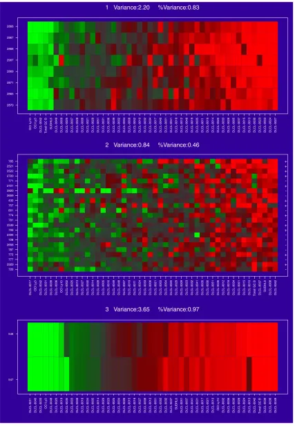
The first three gene clusters found for the DLCL data. Each is a collection of genes showing similar and strong (high variance) expression behavior.

1 Variance:2.20 %Variance:0.83

OCI L

y10

OCI L

y3

DLCL-0042 Tonsil GC B

SUDHL6

DLCL-0049 DLCL-0009 DLCL-0025 DLCL-0007 DLCL-0028 DLCL-0006 DLCL-0021 DLCL-0029 DLCL-0051 DLCL-0031 DLCL-0036 DLCL-0039 DLCL-0002 DLCL-0004 DLCL-0008 DLCL-0052 DLCL-0010 DLCL-0032 DLCL-0034 DLCL-0017 DLCL-0040 DLCL-0001 DLCL-0041 DLCL-0018 DLCL-0012 DLCL-0048 DLCL-0019 DLCL-0035 DLCL-001

1

DLCL-0016 DLCL-0014 DLCL-0020 DLCL-0033 DLCL-0026 DLCL-0005 DLCL-0037 DLCL-0015 DLCL-0013 DLCL-0030 DLCL-0023 DLCL-0003 DLCL-0024 DLCL-0027

2870 2865 2871 2869 2907 2868 2867 2866

2 Variance:0.84 %Variance:0.46

-+ -+ -+ + -+ -+ + -+ -+ + + +

DLCL-0017

OCI L

y3

DLCL-0042 DLCL-0031 DLCL-0039 DLCL-0036 OCI L

y10

DLCL-0002 DLCL-0025 DLCL-0013 DLCL-0027 DLCL-0040 DLCL-0014 DLCL-0028 DLCL-0005 DLCL-0016 DLCL-0049 DLCL-0048 DLCL-0007 DLCL-0019 DLCL-001

1

DLCL-0024 DLCL-0033 DLCL-0006 DLCL-0021 DLCL-0003 DLCL-0004 DLCL-0020 DLCL-0029 DLCL-0009 DLCL-0023 DLCL-0032 DLCL-0041 DLCL-0035 DLCL-0030 DLCL-0051 DLCL-0026 DLCL-0012 DLCL-0018 DLCL-0034 DLCL-0001 DLCL-0015 DLCL-0010 Tonsil GC B DLCL-0037

SUDHL6

DLCL-0008 DLCL-0052

720 2929 777 772 787 2656 728 2494 793 2539 781 774 801 757 432 2659 2820 2721 771 2720 2522 2521 785

3 Variance:3.65 %Variance:0.97

DLCL-001

1

DLCL-0040 DLCL-0033

OCI L

y3

DLCL-0048 DLCL-0020 DLCL-0019 DLCL-0035 DLCL-0003 DLCL-0008 DLCL-0016 DLCL-0034 DLCL-0005 DLCL-0014 DLCL-0029 DLCL-0023 DLCL-0025 DLCL-0004 DLCL-0026 DLCL-0015 DLCL-0018 DLCL-0027 DLCL-0009 DLCL-0012 DLCL-0001 DLCL-0052 DLCL-0032 DLCL-0037

SUDHL6

DLCL-0051 DLCL-0007 DLCL-0041 DLCL-0031 DLCL-0017 DLCL-0021 DLCL-0010 OCI L

y10

DLCL-0002 DLCL-0006 DLCL-0030 DLCL-0028 DLCL-0024 DLCL-0013 DLCL-0042 Tonsil GC B DLCL-0039 DLCL-0036 DLCL-0049

studies, which often consist of millions of measurements. A variety of clustering techniques have been applied to such data, and have proved useful for identifying biologically

relevant groupings of genes and samples [1-13]. Although the underlying principles and computational details of these methods differ, they share the goal of organizing the

comment

reviews

reports

deposited research

interactions

information

refereed research

Figure 4

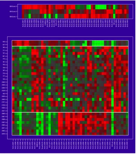
The top panel shows the three signed-mean genes together, and ordered by a hierarchical clustering in this three-dimensional space. The lower panel is similar, except here we show all the genes in each cluster, 33 in all.

DLCL-0041 DLCL-0028 DLCL-0049 DLCL-0042 DLCL-0002 DLCL-0036 DLCL-0039 DLCL-0031 DLCL-0010 DLCL-0051

SUDHL6

DLCL-0009 Tonsil GC B DLCL-0032 DLCL-0025 OCI L

y10

DLCL-0021 DLCL-0006 DLCL-0007 DLCL-0027 DLCL-0030 DLCL-0017 DLCL-0013 DLCL-0024 DLCL-0016 DLCL-0003 DLCL-0014 DLCL-0005 DLCL-0023 DLCL-0035 DLCL-0040 DLCL-0037 DLCL-0026 DLCL-0019 DLCL-0033 DLCL-0048 DLCL-001

1

DLCL-0020 DLCL-0015 DLCL-0034 DLCL-0012

OCI L

y3

DLCL-0008 DLCL-0018 DLCL-0052 DLCL-0004 DLCL-0001 DLCL-0029

SM Gene 1 SM Gene 2 SM Gene 3

DLCL-0041 DLCL-0028 DLCL-0049 DLCL-0042 DLCL-0002 DLCL-0036 DLCL-0039 DLCL-0031 DLCL-0010 DLCL-0051

SUDHL6

DLCL-0009 Tonsil GC B DLCL-0032 DLCL-0025 OCI L

y10

DLCL-0021 DLCL-0006 DLCL-0007 DLCL-0027 DLCL-0030 DLCL-0017 DLCL-0013 DLCL-0024 DLCL-0016 DLCL-0003 DLCL-0014 DLCL-0005 DLCL-0023 DLCL-0035 DLCL-0040 DLCL-0037 DLCL-0026 DLCL-0019 DLCL-0033 DLCL-0048 DLCL-001

1

DLCL-0020 DLCL-0015 DLCL-0034 DLCL-0012

OCI L

y3

DLCL-0008 DLCL-0018 DLCL-0052 DLCL-0004 DLCL-0001 DLCL-0029

elements under consideration (such as genes) into groups (clusters) with coherent behavior across relevant measure-ments (such as samples). Generally absent is any consider-ation of the nature of the coherent variconsider-ation. For example, one might want to identify groups of genes that have coher-ent patterns of expression with large variance across samples, or groups of genes that optimally separate samples into predefined classes (such as different clinical

response groups in tumor samples). Here, we introduce a new statistical method, which we call gene shaving, that attempts to identify groups of elements (genes) that have coherent expression and are optimal for various properties of the variation in their expression.

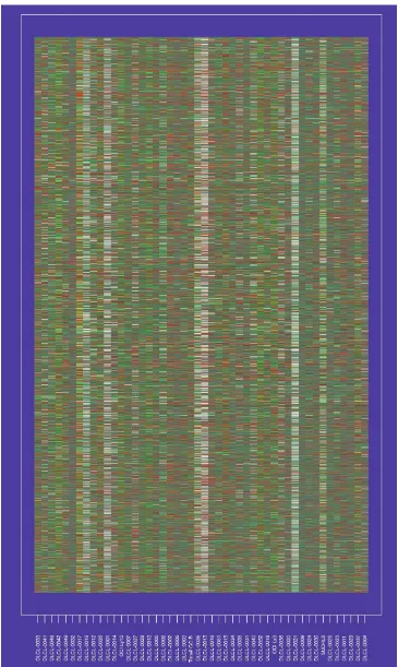
Figure 1 shows the dataset used in our study, which con-sisted of 4673 gene expression measurements on 48 patients

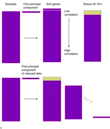
Figure 5

Schematic of the gene shaving process.

Samples

Sort genes

Low

correlation

High

correlation

Shave off 10%

First principal

component

with diffuse large B-cell lymphoma (DLCL). These data have been described in detail previously [14]. The column labels refer to different patients, and the rows correspond to genes. The order of rows and columns is arbitrary.

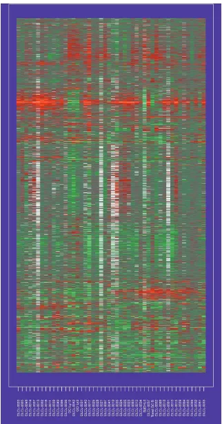
Some authors have recently explored the use of clustering methods to arrange the genes in some systematic way, with similar genes placed close together (see [2] for developments and [15] for an overview). In Figure 2, we have applied hier-archical clustering to the genes and samples separately. Each clustering produces a (non-unique) ordering, one that ensures that the branches of the corresponding dendrogram do not cross. Figure 2 displays the original data, with rows and columns ordered accordingly.

Some structure is evident in Figure 2, and this method can be used to recognize relationships among the genes and samples.

With any method that reduces the dimension of the data, however, finer structure can be lost. For example, suppose the expression of some subset of genes divides the samples in an informative way, correlating with the rate of proliferation of tumor cells, for example, whereas another subset of genes divides the samples a different way, representing the immune response, for example. Then methods such as two-way hierar-chical clustering, which seek a single reordering of the samples for all genes, cannot find such structure.

The method of gene shaving we describe here is designed to extract coherent and typically small clusters of genes that vary as much as possible across the samples. Figure 3 shows three gene clusters for the DLCL data, found using shaving. Some of the genes within each cluster lie close to each other in the hierarchical clustering of Figure 2, but others, and the clusters themselves, are quite far apart.

comment

reviews

reports

deposited research

interactions

information

refereed research

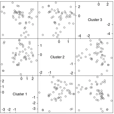
Figure 6

Scatterplot matrix of the three column averages, or ‘super genes’, from each cluster.

-3 -2 -1

0 1 2

0

1

2

-3

-2

-1

Cluster 1

-2

-1

0

1

0

1

-2

-1

Cluster 2

-4

-2

0

2

0

2

In Figure 3 the samples have been ordered by values of the average gene expression. This average gene is a good repre-sentative of the cluster, as all the members are so similar. The variance measures at the top of each cluster are dis-cussed in more detail later. The clusters are all of different sizes. We use an automatic method for determining the size of the clusters, based on a randomization procedure that protects us from looking too hard in the large sea of genes and finding spurious structure. The three cluster-average genes, one from each cluster, are reasonably uncorrelated (see below and Figure 6). This is another aspect of the shaving process - it seeks different clusters, where difference is measured by correlation of the cluster mean. Figure 4 shows the results of a hierarchical clustering applied to the three column-average genes. Whereas hierarchical cluster-ing suggests two main gene groupcluster-ings, the shavcluster-ing process may suggest more useful groupings.

This article is organized as follows. In the section ‘Gene shaving’ we describe the method itself. The section entitled ‘The gap estimate of cluster size’ outlines the gap test for choosing the cluster size. In the section ‘Predicting patient survival’ we try to predict patient survival from gene cluster averages. ‘Supervised shaving’ is discussed in the following

section. Finally, in the ‘Conclusions’ we propose some further generalizations. A more statistical treatment of gene shaving is given in [16].

Results

Gene shaving

In this section we describe in detail our technique for finding clusters like the example in Figure 3. A gene expression matrix is an N×p matrix of real-valued measurements

X=xij. The rows are genes, the columns are samples, and xij

is the measured (log) expression, relative to a baseline. Typi-cally there are missing entries in X. We use a technique described in [17], an iterative algorithm based on the singular value decomposition, for imputing missing expression values; our analysis here assumes that Xhas no missing values. Let Skbe the indices of a cluster of kgenes, and

1 1 1

x–Sk=

be the collection of p column averages of the expression values for this cluster. Then for each cluster size k, gene shaving seeks a cluster Skhaving the highest variance of the

column averages: 1. Start with the entire expression matrix X, each row

centered to have zero mean.

2. Compute the leading principal component of the rows of X.

3. Shave off the proportion α(typically 10%) of the genes having smallest absolute inner-product with the leading principal component.

4. Repeat steps 2 and 3 until only one gene remains. 5. This produces a nested sequence of gene clusters

SN 傻 Sk 傻S_k1傻 S_k2傻 • • • 傻 S1 where Skdenotes a

cluster of kgenes. Estimate the optimal cluster size k^

using the gap statistic described in the section on the gap estimate.

6. Orthogonalize each row of Xwith respect to x–Sk^, the

average gene in Sk^.

7. Repeat steps 1-5 above with the orthogonalized data, to find the second optimal cluster. This process is continued until a maximum of M clusters are found, where Mis chosen a priori.

Box 1

The shaving algorithm.

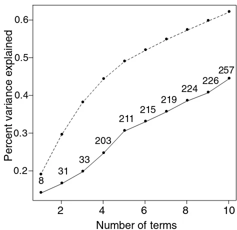
Figure 7

Percent of gene variance explained by first jgene shaving

column averages (j = 1,2, … 0) (solid curve), and by first j

principal components (broken curve). For the shaving

results, the total number of genes in the first jclusters is

also indicated.

Number of terms

Percent variance explained

2

4

6

8

10

0.2 0.3 0.4 0.5 0.6

8 31

33 203

211 215

219

Skmaximizes Var(x–S_k) (1)

The important question of how to choose the cluster size kis addressed in the next section.

Our procedure generates a sequence of nested clusters Sk, in

a top-down manner, starting with k=N, the total number of genes, and decreasing down to k= 1 gene. At each stage the largest principal component of the current cluster of genes is computed. This eigen gene is the normalized linear combination of genes with largest variance across the samples. We then compute the inner product (essentially the correlation) of each gene with the eigen gene, and discard (‘shave off’) a fraction of the genes having lowest (absolute) inner product. The process is repeated on the reduced cluster of genes. The shaving algorithm is depicted in Figure 5 and given in detail in Box 1.

There are a number of duplicate genes in the dataset. In some cases the sequence for a given gene appears on the microarray more than once, either by design or by acci-dent. In other cases, more than one different EST (expressed sequence tag) is present for the same gene. Gene shaving can be affected by duplicate genes, since they are highly correlated with each other. We therefore aver-aged expression profiles for the duplicate genes, leaving 3624 unique gene profiles.

The sequence of operations 1-5 in Box 1 gives the first cluster of rows - the first ribbon in Figure 3. Step 6 orthogonalizes the data to encourage discovery of a different (uncorrelated) second cluster. Note that although we work with the orthog-onalized matrix in the shaving process for the second and subsequent clusters, the derived clusters and their averages involve the original genes.

comment

reviews

reports

deposited research

interactions

information

refereed research

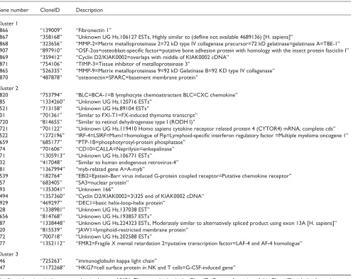
The three gene clusters from unsupervised shaving

Gene number CloneID Description Cluster 1

2866 “139009” “Fibronectin 1”

2867 “358168” “Unknown UG Hs.106127 ESTs, Highly similar to (defline not available 4689136) [H. sapiens]”

2868 “323656” “MMP-2=Matrix metalloproteinase 2=72 kD type IV collagenase precursor=72 kD gelatinase=gelatinase A=TBE-1” 2907 “897910” “OSF-2os=osteoblast-specific factor=putative bone adhesion protein with homology with the insect protein fasciclin I” 2869 “359412” “Cyclin D2/KIAK0002=overlaps with middle of KIAK0002 cDNA”

2871 “754106” “TIMP-3=Tissue inhibitor of metalloproteinase 3”

2865 “526335” “MMP-9=Matrix metalloproteinase 9=92 kD Gelatinase B=92 KD type IV collagenase” 2870 “487878” “osteonectin=SPARC=basement membrane protein”

Cluster 2

2820 “753794” “BLC=BCA-1=B lymphocyte chemoattractant BLC=CXC chemokine” 785 “1334260” “Unknown UG Hs.120716 ESTs”

2521 “713158” “Unknown UG Hs.89104 ESTs”

801 “701361” “Similar to FXI-T1=FX-induced thymoma transcript” 2720 “814655” “Similar to retinol dehydrogenase type I (RODH I)”

2721 “701122” “Unknown UG Hs.119410 Homo sapiens cytokine receptor related protein 4 (CYTOR4) mRNA, complete cds” 2522 “1272196” “IRF-4=LSIRF=Mum1=homologue of Pip=Lymphoid-specific interferon regulatory factor =Multiple myeloma oncogene 1” 2659 “685177” “PTP-1B=phosphotyrosyl-protein phosphatase”

774 “701606” “CD10=CALLA=Neprilysin=enkepalinase” 771 “1305913” “Unknown UG Hs.106771 ESTs”

432 “417048” “Similar to human endogenous retrovirus-4” 781 “1367994” “myb-related gene A=A-myb”

2539 “182764” “EBI2=Epstein-Barr virus induced G-protein coupled receptor=Putative chemokine receptor” 757 “683405” “SA3=nuclear protein”

793 “1353041” “Unknown 166”

2494 “1357360” “Cyclin D2/KIAK0002=3\325 end of KIAK0002 cDNA” 2929 “469297” “DEC1=basic helix-loop-helix protein”

728 “1338981” “Unknown UG Hs.137038 EST” 2656 “814768” “Unknown UG Hs.193857 ESTs”

787 “1338448” “Unknown UG Hs.224323 ESTs, Moderately similar to alternatively spliced product using exon 13A [H. sapiens]” 720 “815539” “JAW1=lymphoid-restricted membrane protein”

772 “700718” “Unknown UG Hs.202588 ESTs”

777 “1352112” “FMR2=Fragile X mental retardation 2=putative transcription factor=LAF-4 and AF-4 homologue” Cluster 3

546 “725263” “immunoglobulin kappa light chain”

547 “1172268” “HKG7=cell surface protein in NK and T cells=G-CSF-induced gene”

The shaving process requires repeated computation of the largest principal component of a large set of variables. If naively implemented, this requires the construction of a

N×N sample covariance matrix Σ of the genes, and the computation of its largest eigenvector. We can avoid the computational burden by working in the dual space, where the matrices have dimension p×p. Furthermore, as we require only the largest eigenvector, the computations can be reduced even further by using the power method, using the eigenvector of the previous cluster as a starting value.

The three resulting clusters are shown in Figure 3 and again in Figure 4. Figure 6 shows the pairwise scatterplots of each of the three column averages (‘super genes’) from the clus-ters. The absolute correlations range from 0.27 to 0.68. The full gene names for the members of the first three clusters are given in Table 1.

It is useful to evaluate how much of the dimensionality of the gene expression variation is captured by the clusters derived from gene shaving. We can approximate the expression

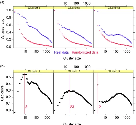
Figure 8

(a) Variance plots for real and randomized data. The percent variance explained by each cluster, both for the original data,

and for an average over three randomized versions. (b)Gap estimates of cluster size. The gap curve, which highlights the

difference between the pair of curves, is shown.

0.0

0.2

0.4

0.6

0.8

1.0

10

100

1000

Cluster: 2

10

100

1000

Cluster: 3

10

100

1000

Cluster size

V

ariance ratio

Real data

Randomized data

8

0.0

0.1

0.2

0.3

0.4

0.5

Cluster: 1

10

100

1000

23

Cluster: 2

10

100

1000

2

Cluster: 3

10

100

1000

Cluster size

Gap curve

(a)

profile for each gene in the complete dataset as a linear com-bination of the three super genes from each cluster (which are simple averages of the genes in each cluster). The percent variance explained by the first j = 1,2, …10 super genes is shown in Figure 7.

Thus the three gene clusters, involving a total of 33 genes, explain about 20% of the variation. The percent variance explained by the first j principal components (broken curve) exceeds that from gene shaving. Each principal component gives a non-zero weight to all 3624 genes, however.

The gap estimate of cluster size

Each shaving sequence produces a nested set of gene clus-ters Sk, starting with the entire expression matrix and then

proceeding down to some minimum cluster size (typically 1). If we applied this procedure to null data, in which the rows and columns were independent of each other, we could still find some interesting-looking patterns in the resulting blocks. Hence, we need to calibrate this process so that we can differentiate real patterns from spurious ones. Even in the case of real structure, it is unlikely that a distinct set of genes is correct for a cluster, and the rest not. More likely there is a graduation of membership eligibility, and we have to decide where to draw the line. Here we describe a proce-dure based on randomization that helps us select a reason-able cluster size.

Our method requires a quality measure for a cluster. We favor both high-variance clusters, and high coherence

between members of the cluster. As the generation of the cluster sequence was driven strongly by the former, we focus on the latter in selecting a good cluster. By analogy with the analysis of variance for grouped data, we define the follow-ing measures of variance for a cluster Sk:

1 p 1

VW= — —

p j=1 k i僆S_k

1 p

VB= —

p j=1

1 p

VT= — (xij– x–)2 Total Variance (4)

kp i僆S_k j=1

= VW+VB

The between variance is the variance of the (signed) mean gene. The within variance measures the variability of each gene about the cluster average, also averaged over samples. As this can be small if the overall variance is small, a more pertinent measure is the between-to-within variance ratio

VB/VW, or alternatively, the percent variance explained

VB V—W

VB

R2_{= 100 — = ———— (5)}

VT 1+_V

W

—VB

A large value ofR2_{implies a tight cluster of coherent genes.}

This is the quality measure we use to select a cluster from the shaving sequence Sk.

Let Skindex the clusters of a given shaving sequence (with k

being the number of genes). Let Dkbe the R2measure for the

kth member of sequence. We wish to know whether Dk is

larger than we would expect by chance, if the rows and columns of the data were independent.

Let X*b_{be a permuted data matrix, obtained by permuting}

the elements within each row of X. We form Bsuch matrices, indexed by b = 1,2, … B. Let Dk*b be the R2 measure for

cluster Sk*b. Denote by D–k* the average of Dk*bover b. The

Gapfunction is defined by

Gap (k) = Dk– D–k* (6)

We then select as the optimal number of genes that value of

kproducing the largest gap:

k

^

= argmaxkGap(k) (7)

The idea is that at the value k^ the observed variance is the most ahead of expected. Multiple clusters are produced for the

comment reviews reports deposited research interactions information

refereed research

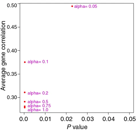
Figure 9

Average (absolute) gene correlation and Cox model p value,

for clusters of size 200 from supervised shaving and for

different values of α. The value of Qa = 0.1 seems best, and

is used in the gene shaving procedure.

P

value

A

verage gene correlation

0.0

0.01

0.02

0.03

0.04

0.05

0.30 0.35 0.40 0.45

0.50 alpha= 0.05

alpha= 0.1

alpha= 0.2

randomized data just like for the original data, and the gap test is used repeatedly to select the cluster size at each stage. For the DLCL data, the maximum for the first cluster occurs at eight genes. Figure 8 shows the percent-variance curves,

Dk, for both the original and randomized tumor data as a

function of size, and the gap curves used to select the specific cluster sizes in Figure 3.

Predicting patient survival

One important motivation for developing gene shaving was the wish to identify distinct sets of genes whose variation in expression could be related to a biological property of the samples. In the present example, finding genes whose expression correlates with patient survival is an obvious challenge. Group factors g1, g2, g3were created by splitting

each gene cluster in Figure 3 into two groups of 24 patients. We used each of these groupings as a factor in Cox’s proportional hazards model for predicting overall survival [18]. Of the group factors only g2was significant,

at the 0.05 level (p =0.04).

In [14], a cluster of 380 genes was chosen on the basis of their large variation over samples, and their ‘germinal center B-like’or ‘activated B-like’ expression profiles. Using these 380 genes, a hierarchical clustering produced two groups of patients which were (just) statistically different in survival. Close inspection shows that 18 of the 23 genes in the second cluster above also fall into this cluster of 380 genes. Hence, gene shaving can find clinically and biologi-cally relevant subdivisions in gene expression data in an unsupervised fashion.

Figure 10

Cluster of 234 genes from supervised shaving.

DLCL-0017 DLCL-0042 DLCL-0021 DLCL-0002 DLCL-0007 DLCL-0040 DLCL-0036 DLCL-0031 DLCL-0006 DLCL-0049 DLCL-0028 DLCL-0048 DLCL-0003 DLCL-0025 DLCL-0012 DLCL-0016 DLCL-0013 DLCL-0018 DLCL-0014 DLCL-0010 DLCL-0039 DLCL-0020 DLCL-0027 DLCL-0004 DLCL-0034 DLCL-0005 DLCL-0051 DLCL-0037 DLCL-0030 DLCL-0001 DLCL-0008 DLCL-001

1

DLCL-0032 DLCL-0052 DLCL-0009 DLCL-0029

It may be fortuitous that one of these groupings correlates with survival, as the clusters were not chosen with survival in mind. We next describe a modification of gene shaving that explicitly looks for clusters that are related to patient survival.

Supervised shaving

The methods discussed so far have not used information about the columns to ‘supervise’ the shaving of rows. Here we gener-alize gene shaving to incorporate full or partial supervision. As in Equation (1), we consider a cluster of genes Skhaving

column average vector x–Sk. Let y= (y1, y2, … yp) be a set of

auxiliary measurements available for the samples. For

example each yjmight be a survival time for the patient

cor-responding to sample jor a class label for each sample, such as a diagnosis category. Supervised shaving maximizes a weighted combination of column variance and an informa-tion measure J(x–Sk,y):

ma

Skx[(1 – α) • Var(x–Sk) + α• J(x–Sk,y)] (8)

for fixed 0≤ α ≤1. The value α= 1 gives full supervision; values between 0 and 1 provide partial supervision.

Choice of the measure J(x–Sk,y) depends on the nature of the

auxiliary information y. If the ycodes class labels, J(x–Sk,y)

comment

reviews

reports

deposited research

interactions

information

refereed research

Figure 11

(a) Gap curve for supervised shaving. (b)Survival curves in the two groups defined by the low or high expression of the 234

genes. Group 1 has high expression of positive genes, and low expression of negative genes; group 2 has low expression of positive genes, and high expression of negative genes. Negative genes are those preceded by a minus sign in Table 2.

Cluster size

Gap curve

1

5 10

50

500

0.0

0.05

0.10

0.15

0.20

0.25

Months

Overall probability of survival

0

20

40

60

80

100

0.0

0.2

0.4

0.6

0.8

1.0

Group 1

Group 2

(a)

(b)

Figure 12

The two groups of samples that showed highest and lowest expression of the gene cluster associated with survival.

DLCL-0017 DLCL-0025 DLCL-0028 DLCL-0031 DLCL-0040 DLCL-0042

DLCL-0049 DLCL-0007 DLCL-0021 DLCL-0006 DLCL-0002 DLCL-0013

DLCL-0016 DLCL-0048 DLCL-0036 DLCL-0012 DLCL-0003 DLCL-0018

DLCL-0039 DLCL-0011 DLCL-0020 DLCL-0027 DLCL-0005 DLCL-0014

DLCL-0030 DLCL-0001 DLCL-0004 DLCL-0008 DLCL-0009 DLCL-0010

DLCL-0029 DLCL-0032 DLCL-0034 DLCL-0037 DLCL-0015 DLCL-0033

Group 1

Cluster from supervised shaving applied to full set of 3624 genes

Position CloneID Description

“-685” “712937” “hPMS1=DNA mismatch repair protein=mutL homologue” “-3531” “1186043” “Unknown UG Hs.134746 ESTs,

“1661” “1352820” “Unknown UG Hs.231825 ESTs” “-2667” “1356433” “Unknown 645”

* “798” “814622” “Unknown UG Hs.49614 ESTs”

“-3545” “713080” “CLK-2=cdc2/CDC28-like protein kinase-2” * “-153” “1339106” “XE7=B-lymphocyte surface protein” * “824” “1356501” “Unknown UG Hs.130721 ESTs”

“-3414” “1319801” “Similar to non-erythropoietic porphobilinogen deaminase (hydroxymethylbilane synt EC4.3.1.8)” “-1577” “1353785” “Unknown UG Hs.119769 ESTs”

“-3242” “376942” “Ro ribonucleoprotein autoantigen (Ro/SS-A)=autoantigen calreticulin”

* “-3535” “1336373” “Similar to High mobility group (nonhistone chromosomal) protein isoforms I and Y” “-3412” “344219” “5’-terminal region of UMK”

“-673” “279363” “Adenosine kinase”

“920” “1355987” “Unknown UG Hs.180836 EST”

* “800” “1358163” “Phosphatidylinositol 3-kinase p110 catalytic, gamma isoform” * “823” “1319062” “WIP/HS PRPL-2=WASP interacting protein”

* “799” “1339726” “Unknown 168” * “788” “825199” “Unknown 164”

“-3544” “1285581” “Similar to myb-related gene A-myb 5’-region”

“-68” “589589” “homolog of Drosophila splicing regulator suppressor-of-white-apricot” * “759” “1333557” “Unknown 161”

“339” “1336946” “Unknown 80”

“-178” “1354703” “Unknown UG Hs.150458 ESTs”

“-933” “1184133” “CASPASE-3=CPP32 isoform alpha=yama=cysteine protease”

“-2714” “149994” “B12 protein=tumor necrosis factor-alpha-induced endothelial primary response gene “-3364” “271976” “ACY1=aminoacylase-1”

“-118” “145409” “Low-affinity IgG Fc receptor II-B and C isoforms (multiple orthologous genes)” * “-671” “1317098” “tyrosine kinase (Tnk1)”

“-2623” “324973” “9G8 splicing factor”

* “783” “814601” “Unknown UG Hs.161905 EST” “2421” “1370055” “Unknown 602”

“1855” “1358160” “Unknown 428”

* “813” “23173” “JNK3=Stress-activated protein kinase” “-1412” “22438” “RYK receptor-like tyrosine kinase” “1104” “1336779” “Unknown 221”

“1521” “1670861” “Unknown UG Hs.32533 ESTs” “2568” “1184568” “Unknown UG Hs.120785 ESTs”

“-3161” “365358” “pM5 protein=homology to conserved regions of the collagenase gene family” “279” “1367883” “KIAA0430”

“338” “1336591” “Unknown UG Hs.180644 ESTs” * “63” “746300” “Unknown UG Hs.136345 ESTs” * “-2661” “1302032” “Deoxycytidylate deaminase”

* “787” “1338448” “Unknown UG Hs.224323 ESTs, Moderately similar to alternatively spliced product exon 13A [H.sapiens]” “2567” “1354788” “Unknown 627”

* “758” “1333558” “Unknown 160” “-3264” “704732” “Unknown 699”

“-2654” “724397” “lymphopain=C1 peptidase expressed in natural killer and cytotoxic T cells”

“1132” “1354522” “Unknown UG Hs.125285 ESTs, Highly similar to (defline not available 4200446) [Mlus]” * “-1595” “1186040” “Unknown UG Hs.136589 ESTs”

“-2320” “241481” “CASPASE-10=Mch4=FLICE2”

“-3345” “502761” “Phosphoribosylglycinamide formyltransferase, phosphoribosylglycinamide synthetase phoribosylaminoimidazole synthetase” “-33” “268727” “MYH=DNA mismatch repair protein=mutY homologue”

* “774” “701606” “CD10=CALLA=Neprilysin=enkepalinase” “-533” “276483” “(2’-5’) oligoadenylate synthetase E” “1388” “1350824” “Unknown UG Hs.163773 ESTs”

“-3244” “488754” “DAP-1=putative mediator of the gamma interferon-induced cell death” “3097” “686331” “DCHT=Similar to rat pancreatic serine threonine kinase”

“-2641” “1355868” “Unknown 643”

“-3135” “199018” “P120=proliferating-cell nucleolar protein” “-1578” “713301” “Unknown UG Hs.32218 ESTs,

“-2502” “153355” “LD78 beta=almost identical to MIP-1 alpha=chemokine”

comment

reviews

reports

deposited research

interactions

information

refereed research

Continued

Position CloneID Description

“2328” “1341026” “yotiao=protein of neuronal and neuromuscular synapses that interacts with specific variants of NMDA receptor subunit NR1” “1863” “1357676” “Unknown UG Hs.191211 ESTs”

“1399” “1356420” “Unknown UG Hs.207995 ESTs”

“-3401” “844479” “Pig8=p53 inducible gene=etoposide-induced mRNA=Similar to E124 = p53 responsive (sculus)” “-3040” “1368740” “Unknown UG Hs.125307 EST”

“-3193” “152653” “C-1-Tetrahydrofolate Synthase, cytoplasmic” “-3437” “814765” “kinase A anchor protein”

“1387” “1318821” “Unknown UG Hs.108614 Homo sapiens mRNA for KIAA0627 protein, partial cds” “-2527” “1357085” “Acidic 82 kDa protein”

* “1400” “682995” “Unknown 298”

* “724” “1286796” “Unknown UG Hs.61506 ESTs” “413” “1334297” “Unknown 98”

* “789” “825217” “Unknown UG Hs.169565 ESTs,

“-2754” “1318136” “5’-AMP-activated protein kinase, gamma-1 subunit” “1052” “1240803” “Unknown 211”

“278” “815671” “Unknown UG Hs.101340 ESTs”

“-2501” “346550” “MIP-1 alpha=LD78 alpha=pAT464=Small inducible cytokine A3=macrophage inflammatory in (G0S19-1)=chemokine” “1988” “1320268” “Unknown 480”

“-903” “704637” “Unknown UG Hs.5354 ESTs” “-2649” “181998” “NFAT3=NFATc4”

“-2648” “171693” “Lst-1=IC7=interferon-gamma-inducible gene present in lymphoid tissues, T cells, macrophages, and histiocyte cell lines encoding a transmembrane protein”

“2373” “1338072” “Unknown 592” “223” “1352327” “Unknown 52” “1269” “1339210” “Unknown 261”

“-3004” “1289545” “Unknown UG Hs.187869 ESTs” “1177” “700949” “Similar to myosin-IXb” * “779” “703735” “Unknown UG Hs.28355 ESTs” * “464” “685761” “Unknown 111”

“1229” “700643” “Unknown UG Hs.104492 ESTs” “-3482” “51058” “E2F-4=pRB-binding transcription factor”

“-3584” “1358191” “Similar to DNA polymerase beta=DNA alkylation repair protein” * “-429” “35356” “Neurotrophic tyrosine kinase, receptor, type 3 (TrkC)”

“-3136” “265590” “NF1=Neurofibromin” “956” “1289384” “Unknown 198”

“2491” “814251” “SLAM=signaling lymphocytic activation molecule” “2083” “1353083” “Unknown UG Hs.136972 EST”

“1102” “1372068” “KIAA0603=Similar to TBC1” “-1010” “595474” “Pak1=p21-activated protein kinase” “-3594” “1269836” “BCL-7B”

“-2270” “265267” “HSP70”

“-944” “1337124” “Unknown UG Hs.81248 CUG triplet repeat, RNA-binding protein 1” “-3330” “1301224” “Elongin B=RNA polymerase II transcription factor SIII p18 subunit” “1658” “1241118” “Unknown 346”

“-3140” “841361” “GRO2=GRO beta=MIP2 alpha=macrophage inflammatory protein-2 alpha=chemokine” “-2651” “525540” “BCL-3”

“-3350” “1186114” “Unknown UG Hs.116447 EST” “-2990” “1289569” “Unknown UG Hs.146165 ESTs”

* “809” “1270618” “Unknown UG Hs.208970 EST, Weakly similar to neuronal thread protein AD7c-NTP [ens]” “-3160” “703707” “Protein disulfide isomerase-related protein (PDIR)”

“874” “1320313” “Unknown UG Hs.132458 ESTs” “-3390” “1339763” “Unknown 710”

“1343” “1318717” “LOK=lymphocyte oriented kinase=STE20-like protein kinase that is expressed predominantly in lymphocytes” “-179” “301551” “Integrin, alpha V (vitronectin receptor, alpha polypeptide, antigen CD51)”

* “723” “824754” “Unknown UG Hs.145058 ESTs”

“-3406” “1300230” “Unknown UG Hs.56421 ESTs, Weakly similar to Similarity to H.influenza ribonucl H [C.elegans]” “-573” “1341161” “Similar to rhoGap protein”

* “722” “1341225” “Unknown UG Hs.186709 ESTs,! [H.sapiens]” “2212” “1350784” “Unknown UG Hs.163202 EST”

“-3478” “417897” “cleavage stimulation factor 77kDa subunit=polyadenylation factor subunit=homolog the Drosophila suppressor of forked protein”

“-887” “756965” “RGS14=regulator of G protein signaling”

Continued

Position CloneID Description

“1344” “825333” “Unknown UG Hs.193017 ESTs, Highly similar to (defline not available 4220898) [ens]” * “743” “1358192” “Unknown UG Hs.228205 EST,

“1850” “1353072” “Unknown 426”

“-3391” “1340604” “Unknown UG Hs.127121 ESTs” “-236” “686771” “tubulin-gamma”

“-3343” “293934” “CAS=chromosome segregation gene homolog” “2566” “1350728” “Unknown 626”

“-2984” “955354” “putative cell surface ligand for T1/ST2 receptor (related to IL-1 receptors)” “-3149” “366713” “GSK3=glycogen synthase kinase 3”

* “720” “815539” “JAW1=lymphoid-restricted membrane protein”

“-3177” “378364” “PRODH=proline dehydrogenase/proline oxidase=p53-induced gene” “1268” “1339305” “Unknown 260”

“-3616” “1302092” “Unknown UG Hs.214428 ESTs” “1210” “685368” “Unknown 243”

“2330” “1240688” “Unknown 577”

“259” “1369262” “KIAA0019=similar to transforming protein tre”-2528” “1184411” “MINOR=mitogen induced nuclear orphan receptor=NOR-1=Nur77 orphan nuclear receptor family member”

“-3586” “1309295” “Unknown UG Hs.136985 ESTs” “2045” “1352570” “Unknown 494”

“2067” “1320316” “Unknown 508” “-3533” “298303” “TECK chemokine”

“-3530” “1355240” “Unknown UG Hs.130849 ESTs” * “-2469” “417226” “c-myc”

“1784” “1355354” “Unknown 394”

“-3023” “700772” “Smad2=Madr2=JV18-1=Homologue of Mothers Against Decapentaplegic (MAD)=Activated beta” * “793” “1353041” “Unknown 166”

“-3162” “1289546” “Similar to arginine/aspartate-rich 37.3K protein” * “-2669” “1186215” “Unknown UG Hs.190288 EST”

“-113” “1337185” “KIAA0037”

“-3434” “1338032” “CPR2=cell cycle progression 2” “-2621” “1338456” “c-myc binding protein”

“1333” “824376” “Similar to (AF016450) Similar to acyltransferase”

“-3405” “1334813” “Unknown UG Hs.17883 protein phosphatase 1G (formerly 2C), magnesium-dependent, isoform” “2301” “300051” “myosin light chain-2”

“1144” “1372011” “Unknown UG Hs.209146 ESTs”

“-3436” “485171” “methionine adenosyltransferase alpha subunit” “1339” “1355713” “Unknown 277”

“1156” “1351290” “Similar to (Z49125) C47G2.4” * “721” “1353015” “Unknown 154”

“-3125” “86040” “Cytochrome P450, subfamily I, polypeptide 2 (aromatic compound-inducible)” “258” “1367988” “Unknown 61”

“-3258” “1304523” “APRT=adenine phosphoribosyltransferase” “-3548” “1340120” “Unknown 733”

“1511” “1351701” “Unknown UG Hs.124230 ESTs” “-3280” “826594” “replication factor C”

“-3363” “293035” “APEX=apurinic endonuclease=DNA alkylation repair protein” “1190” “1371313” “Similar to G-protein coupled receptor pH218”

“1321” “1309301” “Unknown UG Hs.136987 EST”

“-3180” “591683” “GADD45 alpha=growth arrest and DNA-damage-inducible protein alpha” “1748” “1371159” “Unknown 377”

“-2781” “1288183” “BAK=BCL-2 family member” “108” “1370125” “Unknown 22”

“-2941” “742132” “Interferon-induced 17 KD protein” “-2994” “1271685” “Unknown UG Hs.176669 ESTs”

“1287” “1353226” “Unknown UG Hs.30209 Homo sapiens mRNA for KIAA0854 protein, complete cds” “1039” “1671442” “Unknown UG Hs.171096 ESTs, Weakly similar to (defline not available 4456988) [ens]” * “83” “52408” “ABR=guanine nucleotide regulatory protein”

“3624” “1355859” “Similar to myosin IE heavy chain” “-2746” “1350736” “IRF-3=interferon regulatory factor-3” “1303” “665682” “Jnkk2=JNK kinase 2=MAP kinase kinase” “877” “1367968” “Unknown UG Hs.105072 ESTs” “-3344” “1341245” “CD73=5’ nucleotidase”

can be taken as the sum of squared differences between the category averages x–Sk. For censored survival times y, think of

x–Skas a covariate in a Cox (proportional hazards) model. If

the score vector from this model is g, we set J(x–S_k,y) = ggT,

a p×pmatrix. Computationally we first scale the genes so that the within-risk set variance is 1.

When fully supervised, the shaving procedure reduces to simply ranking the genes from largest to smallest Cox model score test. Thus there is no role for principal components or top-down shaving in this case. However, to encourage coher-ence within the gene clusters, it can be better to use a partially supervised criterion, which does use principal components

comment

reviews

reports

deposited research

interactions

information

refereed research

Continued

Position CloneID Description

“1191” “1371317” “Similar to arylacetyltransferase” * “-310” “154493” “HNPP=nuclear phosphoprotein” “1976” “1334933” “Unknown UG Hs.144684 ESTs”

“-2609” “1670958” “SRF=c-fos serum response element-binding transcription factor” “405” “701689” “putative tumor suppressor (LUCA15)”

“-3319” “1307997” “Similar to bromodeoxyuridine-sensitive transcript protein=px19” “-3255” “810743” “MLF2=myelodysplasia/myeloid leukemia factor 2”

“2150” “1353466” “Unknown UG Hs.124360 EST”

“-2650” “511407” “69 kDa 2’5’ oligoadenylate synthetase (P69 2-5A synthetase)”

“252” “1356345” “Unknown UG Hs.49500 Homo sapiens mRNA for KIAA0746 protein, partial cds” “1337” “1367875” “Unknown UG Hs.128127 ESTs”

“1302” “1351266” “Unknown UG Hs.134197 ESTs, Moderately similar to FAM [M.musculus]” “1386” “815165” “Unknown UG Hs.188732 ESTs”

“-3147” “549277” “cell cycle protein p38-2G4 homolog (hG4-1)” “-3349” “1355524” “Similar to rapamycin-binding protein (FKBP25)”

“-173” “1287032” “Similar to Drosophila female sterile homeotic (FSH) homologue”

* “777” “1352112” “FMR2=Fragile X mental retardation 2=putative transcription factor=LAF-4 and AF-4 ogue” “-3334” “346948” “nm23-H2=NDP kinase B=Nucleoside dephophate kinase B”

“-3256” “1303575” “Unknown UG Hs.123304 ESTs” “1289” “704690” “Dyrk6=Ser/Thr protein kinase” “1133” “1351498” “Unknown UG Hs.189063 ESTs” “2058” “1339890” “Unknown 503”

“-2927” “342647” “MAPKAP kinase (3pK)” “1324” “687198” “Unknown UG Hs.125860 ESTs”

“-3047” “203704” “flavin-containing monooxygenase (FMO1)”

“-2662” “1288102” “Similar to nuclear-encoded mitochondrial NADH-ubiquinone reductase 24Kd subunit” “1852” “1371200” “Similar to (Z78012) C52E4.6”

“1383” “1319529” “Unknown 293”

“-3360” “1671396” “Similar to friend of GATA-1 (FOG)=zinc finger GATA-1 coactivator in erythroid and megakaryocyte lineages” “1228” “1336501” “Unknown 249”

“1353” “1356762” “Unknown UG Hs.127480 ESTs” * “-575” “490387” “zinc finger protein 42 MZF-1” “1242” “1031754” “Protein-tyrosine phosphatase 2C” “1211” “1372274” “Unknown UG Hs.208983 ESTs,

“-2759” “489438” “MyD88=myeloid differentiation primary response protein=death domain-containing p “1227” “1334962” “Similar to KIAA0437”

“260” “1341211” “Unknown UG Hs.191209 ESTs”

“-3137” “1250770” “Purine nucleoside phophorylase=Inosine phosphorylase=PNP” “1385” “1371029” “Unknown 295”

“1808” “1372833” “Unknown 403”

“-2762” “1184153” “Unknown UG Hs.230206 EST” “1046” “1352940” “Unknown 208”

“-2766” “756452” “tyk2=non-receptor protein tyrosine kinase” “1204” “1370570” “Lamin B receptor (LBR)”

“1201” “1241671” “Similar to (AE000860) conserved protein [Methanobacterium thermoautotrophicum]” * “735” “686893” “Unknown UG Hs.226955 ESTs”

“1338” “1370103” “Unknown 276”

“255” “1338624” “Unknown UG Hs.192864 ESTs” “1200” “1352335” “Unknown UG Hs.99701 ESTs”

“2133” “1340880” “Cancer associated surface antigen (RCAS1)”

and top-down shaving. This is demonstrated in the example below. One can also include other prognostic factors in the model, and direct shaving to find a gene cluster whose column average is a strong predictor in the model. This can be done with other models, for example a linear regression model for a quantitative measurement. Operationally, all of these choices for Jare quadratic functions of the column averages x–S_k, and

gene shaving can be carried out via principal components of a suitably modified variance matrix.

We applied supervised shaving to the set of 3624 genes from the DLCL samples. Figure 9 examines the effect of different values of the supervision weight α, showing the average (absolute) gene correlation and Cox model pvalue for each choice. From this plot we chose the value α= 0.10, which gives a good mix of high gene correlation and low p value. Partially supervised gene shaving pro-duced a cluster with 234 genes, shown in Figure 10 and in Table 2.

Figure 13

Supervised gene shaving from full gene set. (a,c)Partially supervised with α= 0.10; (b,d)fully supervised (α= 1). (a,b)

Training set p values; (c,d) permutation p values for the cluster average as a function of cluster size. The chosen cluster size of

234 is indicated.

Cluster size

p

value

1

5

50

500

0.0

0.0010

0.0020

(a)

Partially supervised

Cluster size

1

5

50

500

0.0

0.0010

0.0020

(b)

Fully supervised

Cluster size

p

value

p

value

p

value

1

5

50

500

0.0

0.04

0.08

0.12

(c)

Partially supervised

Cluster size

1

5

50

500

0.2

0.4

0.6

0.8

Some of the genes are close together in the hierarchical clus-tering order (indicated by the first number in Table 2), many are not. Some genes have a negative sign, and others have no sign. We will call these ‘negative’ and ‘positive’ genes respec-tively. The negative genes have their expression values flipped before being averaged with other gene expression profiles. Figure 11a shows the gap curve, suggesting a cluster size of 35. However, further analysis below suggests the better cluster size of 234.

The cluster of 234 genes contains many of the strongest indi-vidual genes for predicting survival. For example, 130 of the strongest 200 genes are in the cluster. Some weaker genes are, however, also in the cluster, the weakest being the 1332nd strongest gene among the full list of 3624. Figure 11b shows the survival curves stratified by the low and high expression of this gene cluster, using the median of the cut-off point. The two resulting groups are shown in Figure 12.

Using this grouping as a predictor in the Cox model for sur-vival gave a highly significant p value (0.00042). However, this p value must be scrutinized. Figure 13a,b shows the Cox model p value as a function of the cluster size, for both par-tially and fully supervised shaving. We will call these the ‘training set p values’. As the gene shaving process was supervised by the survival times, the training set p values will be biased downward, and it is important to adjust them appropriately. We permuted the survival times, re-ran the shaving process and computed the corresponding p values. This was repeated 100 times, and for each cluster size we computed the proportion of times the permutation p values were less than or equal to the training set p values. These proportions are shown in Figure 13c,d, and are unbiased estimates of the true p values. Fully supervised shaving is too aggressive, and the upward adjustment of the p values is large. As a result the p value is around 0.05 for the full set of genes, but none of the smaller clusters is significant at the

comment

reviews

reports

deposited research

interactions

information

refereed research

Figure 14

Kaplan-Meier survival curves in the two groups defined by the cluster of 234 genes shown in Figure 10, stratified by IPI. Group 1 has high expression of positive genes and low expression of negative genes in Figure 9, and vice-versa for Group 2.

Months

Overall probability of survival

Overall probability of survival

0

20

40

60

80

100

0.0

0.2

0.4

0.6

0.8

1.0

Group 2

Group 2

Group 1

Group 1

Low IPI

Months

0

20

40

60

80

0.0

0.2

0.4

0.6

0.8

1.0

High IPI

Table 3

Cross-tabulation of gene shaving groups with IPI index

IPI

Low High

Gene shaving groups

1 7 7

2 11 7

Table 4

A comparison of the patient groups obtained by gene shaving with those obtained previously [14]

Patient groups of Alizadeh et al.[14]

Low High

Gene shaving groups

1 13 5

0.05 level. For partially supervised shaving, many of the p

values are below 0.05, and from this we chose the cluster size of 234 near the minimum.

Using the full set of genes, flipping each to have positive cor-relation with survival, averaging their expression values and finally cutting at the median, gave a grouping nearly the same as Groups 1 and 2 in Figure 12. The only change was a swap between DLCL-0014 and DLCL-0018, and these two samples are right at the median cutpoint between the two groups in Figure 10.

The international prognostic index (IPI) A score was also available for these patients. Components of the IPI include age, level of the enzyme lactate dehydrogenase (LDH) and the number of extranodal sites. As in [14], we dichotomized IPI scores into low (0, 1 or 2) and high (3, 4 or 5). The result-ing groupresult-ing seems to be about as predictive as the IPI index, and is quite independent from it, as Table 3 indicates. When added to a Cox model containing IPI, this grouping had a training set p value of 0.0006. Figure 14 shows the Kaplan-Meier survival curves for each group, stratified by low and high IPI.

In [14], two patient groups were defined from a hierarchical clustering tree grown from a 380-gene cluster. As a predic-tor, the grouping was just significant in the low IPI group only, at the 0.05 level. Table 4 gives a cross-tabulation of that grouping with the one used in this paper in Figure 10. Thus 25/36 = 69% of the patients are classified the same way by both groupings. The patient grouping of Alizadeh et al.

[14] was based on a cluster of 380 genes, chosen for their large variation over the samples. Our cluster of 234 genes has 38 genes in common with this cluster of 380, and they are indicated by an asterisk in Table 2. Five of the 234 genes also appear in the unsupervised clusters found earlier, in the second of the three clusters.

Conclusions

We have proposed a set of ‘shaving’ methods for isolating interesting clusters of genes from a set of DNA microarray experiments. The methods may be unsupervised, or may be supervised - that is, use information available about the samples such as a class label or survival time. The pro-posed shaving methods search for clusters of genes showing both high variation across the samples, and coher-ence (correlation) across the genes. Both of these aspects are important and cannot be captured by simple clustering of the genes, or thresholding of individual genes based on the variation over samples.

With our model-based approach for supervised shaving, one can incorporate other prognostic factors in the search for

interesting gene clusters. If an outcome such as survival time is available for each sample, the method searches for a gene cluster whose column average gene x–has a significant effect, possibly the presence of other prognostic factors, for predict-ing the outcome.

The microarray data xij we have considered are real-valued

expression levels. However, other kinds of arrays produce dif-ferent kinds of data. In particular, some arrays detect the pres-ence or abspres-ence of single-nucleotide polymorphisms (SNPs), so that the xijvalues take on one of k≥2 unordered values.

The shaving methods described can be easily modified to handle this kind of data. In detail, we construct kdata matri-ces X1, X2… Xk, each of size n×m. The ijth element of Xjis 1 if

xijfalls in class j, and zero otherwise. Letting Σj j = 1, 2, … k be

the n×n covariance matrices of the genes in each Xj, we

simply apply principal component shaving, using

the variance matrix for the penalty. This can be done unsuper-vised, or a supervision term can also be added.

Acknowledgements

We thank Mark Segal for helpful discussions, and Nick Fisher and Jerome Friedman for their work on ‘bump-hunting’ which inspired some of the ideas in this paper. The first two authors were supported by grants from The National Science Foundation and the National Institutes of Health. W.C.C. was supported by NIH grant UO1-CA 84967. R.L. and collabora-tors were supported by LPPG grant CA 34233.

References

1. Weinstein J, Myers T, O’Connor P, Friend S, Fornace A Jr, Kohn K, Fojo T, Bates S, Rubinstein L, Anderson N, et al.: An information-intensive approach to the molecular pharmacology of cancer. Science1997, 275:343-349.

2. Eisen M, Spellman P, Brown P, Botstein D: Cluster analysis and display of genome-wide expression patterns.Proc Natl Acad Sci USA 1998, 95:14863-14868.

3. Roth FP, Hughes J, Estep P, Church G: Finding DNA regulatory motifs within unaligned noncoding sequences clustered by whole genome mRNA quantitation. Nat Biotechnol 1998, 16:939-945.

4. Golub T, Slonim D, Tamayo P, Huard C, Gassenbeek M, Mesirov JP, Coller H, Loh M., Downing J, Caligiuri M, Bloomfield C, Lander E: Molecular classification of cancer: class discovery and class prediction by gene expression monitoring. Science 1999, 286:531-538.

5. Perou C, Jeffrey S, van de Rijn M, Rees C, Eisen M, Ross D, Perga-menschikov A, Williams C, Zhu S, Lee J, et al.:Distinctive gene expression patterns in human mammary epithelial cells and breast cancers. Proc Natl Acad Sci USA1999, 96:9212-9217. 6. Alon U, Barkai N, Notterman D, Gish K, Ybarra S, Mack D, Levine

A: Broad patterms of gene expression revealed by clustering analysis of tumor and normal colon tissues probed by oligonucleotide arrays. Proc Natl Acad Sci USA1999, 96:6745-6750.

7. Brazma A, Jonaxsen I, Vilo J, Ukkonen E: Predicting gene regula-tory elements in silico on a genomic scale. Genome Res1998, 8:1202-1215.

8. D’haeseleer P, Wen X, Fuhrman S, Somogyi R: Inferring gene relationships from large-scale gene expression data. In Infor-mation Processing in Cells and Tissues. Edited by Holcombe M, Paton R. New York: Plenum; 1998:203-212.

9. Ewing R, Kahla A, Poirot O, Lopez F, Audic S, Claverie J: Large-scale statistical analyses of rice ESTs reveal correlated pat-terns of gene expression. Genome Res1999, 10:950-959. 10. Mjolsness E, Mann T, Castano R, Wold B: From co-expression to

tory, Section 365;1999.

11. Niehrs C, Pollet N: Synexpression groups in eukaryotes.Nature 1999, 402:483-487.

12. Walker M, Volkmuth W, Sprinzak E, Hodgson D, Klinger T: Predic-tion of gene funcPredic-tion by genome scale expression analysis: prostate cancer associated genes.Genome Res9:1198-1203. 13. Tamayo P, Slonim T, Mesirov J, Zhu Q, Kitareewan S, Dmitrovsky E:

Interpreting patterns of gene expression with self-organiz-ing maps: Methods and applications to hematopoietic diferentation. Proc Natl Acad Sci USA1999, 96:2907-2912. 14. Alizadeh A, Eisen M, Davis RE, Ma C, Lossos I, Rosenwal A, Boldrick

J, Sabet H, Tran T, Yu X et al.:Identification of molecularly and clinically distinct substypes of diffuse large B-cell lymphoma by gene expression profiling. Nature2000, 403:503-511. 15. Tibshirani R, Hastie T, Eisen M, Ross D, Botstein D, Brown P:

Clus-tering methods for the analysis of DNA microarray data. Technical report. Stanford: Department of Statistics, Stanford Uni-versity;1999.

16. Hastie T, Tibshirani R, Eisen M, Brown P, Scherf U, Weinstein J, Alizadeh A, Staudt L, Botstein D:Gene shaving: a new class of clustering methods for expression arrays. Technical report. Stanford: Stanford University; 2000.

17. Hastie T, Alter O, Sherlock G, Eisen M, Tibshirani R, Botstein D, Brown P: Imputation of missing values in DNA microarrays. Technical report. Stanford: Stanford University; in press.

18. Cox D: Regression models and lifetables. J Roy Statist Soc B 1972, 74:187-220.

comment

reviews

reports

deposited research

interactions

information