Determining a Source in Air Dispersion with a Parallel Genetic Algorithm

(1)

International Journal of Emerging Technology and Advanced Engineering

Website: www.ijetae.com (ISSN 2250-2459, ISO 9001:2008 Certified Journal, Volume 7, Issue 8, August 2017)

174

Determining a Source in Air Dispersion with a Parallel Genetic

Algorithm

Frank Gronwald

1

, Shoou – Yuh Chang

2

, An Jin

3

North Carolina A&T State University Civil Engineering Department

Abstract—Today there are many methods of observing the concentration of a pollutant at a particular point. By taking the measurements of several points in a region, a concentration profile can be created. In most of cases, however, it is crucial to identify the sources of the pollution to initiate mitigation procedure. The use of a backwards parallel genetic algorithm (BPGA) is proposed in this study to serve that purpose. The BPGA uses multiple guesses in a generation and through use of a fitness function the best possible guess is used for reproduction of the next generation. Through many generations of this process, the backwards parallel genetic algorithm is able to closely find the coordinates of the source, the amount of the source, and which model was used out of the model pool. The results indicate that the proposed BPGA approach can identify the location and amount of a pollutant source successfully.

Keywords—Air pollution modeling, Parallel Genetic Algorithm, PIKAIA, Parameter Estimation

I. INTRODUCTION

Pollutants such as chemicals, biological or reactive agents, and greenhouse gasses are released from various sources and transported in the air. In most cases, the information of the release sources is unknown or uncertain. This information is crucial for air quality control or dealing with environmental disasters. Today, there are several air quality models which have been developed to simulate the transport of pollutants when given a source. One disadvantage of many models is that the observed data may only be available at certain limited time and space scales (Ayra, 1995).

Low wind dispersion studies play a vital role due to the fact that low wind conditions apply for a majority of the time. It is known that atmospheric dispersion in low wind speed conditions is mainly governed by meandering low frequency horizontal wind oscillations (Allen et al, 2007). In such conditions, the airborne pollutants are generally dispersed over rather wide angular sectors. This causes the low wind dispersion models to work especially well when the dispersion is restricted to a limited area (Agarwal et al, 2005).

During low wind conditions pollutant particles do not travel very far from the source (Ayra, 1995). Low wind conditions are generally present when the wind velocity is below 2 m/s.

The Gaussian plume model is one of the most often used. Under light wind conditions, however, there are some possible deficiencies such as neglecting downwind diffusion in comparison to advection and unavailability of several dispersion parameters (Sharan and Modani, 2005).

The Variable K model was proposed as an improvement of the Gaussian model to deal with low wind dispersion by Sharan and Yadav (1998). It included streamwise diffusion and variable eddy diffusivities. The eddy diffusivities were specified as linear functions of downwind distance. They tested their model against the dispersion data collected by the Idaho National Engineering Laboratory (INEL) and compared the performance of the model using different parameterizations for the eddy diffusivities and varying time intervals of 2 and 60 min (Oetti et al, 2001). It was discovered that by using a time interval of 2 min and a dependency of the eddy diffusivities on measured standard deviations of wind direction fluctuations gave the best results. Sagendorf and Dickson (1974) used a Gaussian model and also divided each computation period into 2-min time intervals and summed the results to determine the total concentration. However, such a model becomes questionable when the chosen time intervals are below the ratio of the maximum travel distance to the average wind speed xmax/u (Oetti et al, 2001).

(2)

International Journal of Emerging Technology and Advanced Engineering

175

II. METHODOLOGY

A. Models

The backwards Parallel Genetic Algorithm is able to use the high calculation power of today’s computers to guess at the answer multiple times. Each generation consists of 64 guesses and the best fit solution is carried over for reproduction. The dispersion model is run at several points in parallel with a set of starting parameters such as the location of the source and a final concentration is obtained. The concentrations are then fed into the backwards PGA and a set of parameters are obtained from which comparisons can be made. The models that will be used are as follows.

The steady state dispersion of a pollutant can be described by the Advection and Dispersion Model, which is given by the equation

S z C K z y C K y x C K x x C

U _x _y _z 

                 ) ( ) ( ) ( (1) where C is the mean concentration (g/

3

m

_{), S is the}

source,

K

x

,

K

y_{, and}

K

_z_{are the eddy diffusion}

coefficients in the x, y, and z directions, and U is the mean wind velocity in the x axis (m). The solution to equation (1) depends on the parameterization of U, K and S. U can either be a constant or a power function of z. The K value can also be a constant or a function of their position. S is based on the position of the source relative to the coordinate system (Sharan and Yadav, 1998). For this study, U is kept constant with a non zero value and the K values are made to be linear functions of downwind distance based on Taylor’s theory for small travel times such that

x

x U

K 



_, Ky 



Uy_, K_z U_z

(2)

where α, β, and



represent turbulence parameters and vary with stability. With this diffusivity parameterization, Equation (1) is transformed to

                                   z C Ux z y C Ux y x C Ux x x C

U   

(3) Under stable conditions,

2 */ ) ( 25 .

6 u U





_,





2

*/ )

( 61 .

3 u U _,

2

*/ )

( 69 .

1 u U





where U is the mean wind velocity and

u

*_{is the friction} velocity scale.

The models used for the experiment were special cases of the Advection Dispersion Model. The No Wind Dispersion Model and the Light Wind Dispersion Model were coded in FORTRAN to be called in the Parallel GA Frame. The first model examined was the No Wind Dispersion Model (Sharan and Yadav, 1998) which was based on isotropic diffusion and no wind velocity (U=0). In this instance the isotropic diffusion was given by the equation:

Kr

Q

C



4 

(4) where r is the radial distance from the source (m), K is

the diffusion constant, and Q is the pollutant emission rate (g/s)

The second model examined was the Light Wind Dispersion Model (Sharan and Yadav, 1998)



Z H Z H



z

y

x

F

x

U

Q

C



_



_

2 )

, , (

2 



(5) where





 1/2 1 2 2 2   

























_













y

z

H

x

F

_z _H (6)





 1/2 1 2 2 2   

























_













y

z

H

x

F

z H

(7) The observation data were obtained from simulation models. The models were run at another site using a set of initial parameters. The concentration was calculated for several points at various distances away from the source.

III. PIKAIAAND GAPROGRAM

(3)

International Journal of Emerging Technology and Advanced Engineering

176

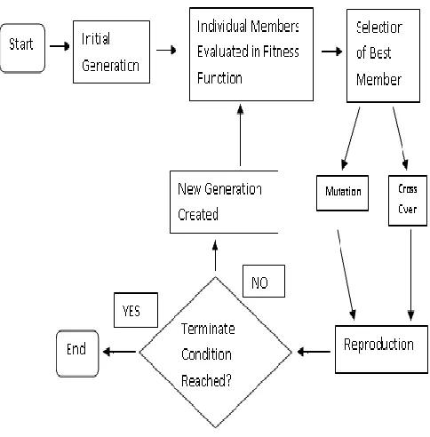
PIKAIA maximizes a specified FORTRAN function through a call in the body of the main program on the multi-node computing unit which can support Message Passing Interface (MPI). PIKAIA uses decimal as opposed to binary encoding. Binary operations are usually carried out through platform-dependent functions in FORTRAN, which makes it more difficult to port the code between the Intel and Sun platforms (Metcalfe 2001).

[image:3.612.50.292.417.663.2]

PIKAIA incorporates only the two basic genetic operators: uniform point crossover, and uniform one-point mutation. The mutation rate can be dynamically adjusted during the evolution, using either the linear distance in parameter-space or the difference in fitness between the best and median solutions in the population. The practice of keeping the best solution from each generation is called elitism, and is a default option in PIKAIA. Selection is based on ranking rather than absolute fitness, and makes use of the Roulette Wheel algorithm. There are three different reproduction plans available in PIKAIA: Steady-State-Delete-Random, Steady-State-Delete-Worst, and Full Generational Replacement. Only the last of these is easily parallelizable. Figure 1 displays the flow chart for the parallel generation algorithm.

Figure 1: Process Chart of a Backwards PGA

A fitness function was run and then the test data were generated with post processing procedures being performed

afterwards. The fitness function was defined as:







o

m

SV

ff

1

(8) where

SV

m_{is the concentration calculated by the model}

and

SV

o_{is the concentration observed at the measuring}

site. The fitness function works to choose the best value which is also closest to the observed value. The objective is to have the model calculate the value obtained at the measuring site. When the two values are equal the fitness function is maximized.

IV. EXPERIMENTS

The goal of these experiments is to inverse out the source term parameters. The testing plan involves running the Models at the source location with fixed parameters to generate output data. The output data is then run through the PGA to guess the set of parameters. Through comparison of the parameters, it will be shown how well the PGA is working and how it can be improved.

The parallel genetic algorithm program, PIKAIA, was tested on a 16 node Linux system. The model was arranged such that the range of x was 0 to 200 m in the eastward direction, y was northward but fixed at zero, and the range of z was upwards between 0 and 300 m. The grid was set so that i ranged from 0 to 40, and k ranged from 0 to 60. The maximum generation was 99 for three parameter estimation and 999 for four parameter generation.

(4)

International Journal of Emerging Technology and Advanced Engineering

[image:4.612.55.289.150.301.2]

177

Figure 2: Process Chart of the Experiments

Testing of the Models

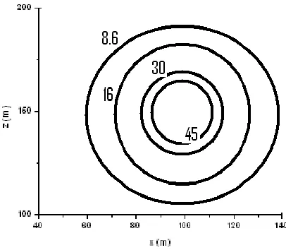
The first two experiments were designed as tests of both the models and backward PGA. In the first experiment three parameters were found inversely from a no-wind data set using 2400 observations. The testing environment consisted of an area with 40 grid points in the x direction and 60 grid points in the z direction. An observation station was placed every grid cell as so called ―Full‖ observation dataset. For all of the experiments it was defined that dx=5m and dz=5m. In the first experiment the source was centered at the point x=100, z=150 and the emission rate was 4 g/s. Figure 3 shows the concentration profile of the pollutant at each observation point. As expected, the highest value occurred at the source and rapidly declined going away from the source. Figure 4 shows the pollutant concentration at the surface level observation points. This time the highest concentration occurred at the source and then decreased slightly with increasing distance.

[image:4.612.342.545.158.335.2]

Figure 3: Pollutant Concentration for Experiment 1

[image:4.612.343.534.376.579.2]

(5)

International Journal of Emerging Technology and Advanced Engineering

[image:5.612.73.254.334.522.2]

178

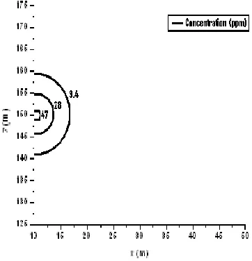
The second experiment was performed as a test of the light wind model. In this instance the size of domain stayed the same but the x coordinate of the source was moved to 0 and the z coordinate was moved to 155 to account for the wind. The source emission rate was increased to 99 g/s. A concentration profile of the pollutant is shown in Figure 5. It shows the concentration of the pollutant decreasing about as rapidly in the x direction as compared to the z direction. The light wind did not significantly affect the distance the particles traveled when compared to the no wind model. This is even more apparent in Figure 6 which shows the pollutant concentration at the surface layer. Since the concentration at the surface level was low to begin with, the drop off from the center was very slight.

Figure 5: Pollutant Concentration (ppm) for Experiment 2

Figure 6: Pollutant Concentration at Surface Layer for Experiment 2

Obtaining the Parameters Using Only the Surface Layer Data

Because of the high cost and impracticality of collecting pollutant concentration at high altitudes most measurement devices are located on the surface. By just using the available sites at the surface level the number of observations will fall to 40. If the models and backwards PGA could correctly calculate the initial parameters using fewer sites they would become even more valuable. The third experiment used only these 40 points from the no wind data set. Figure 4 displays the values obtained at the surface observation points. The concentration values remained exactly the same as in the first experiment.

(6)

International Journal of Emerging Technology and Advanced Engineering

179

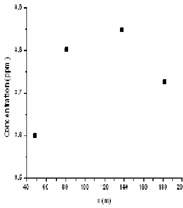
The number of sampling locations was cut from 40 to 4. The experiment focused on estimating three parameters which were the x and z coordinates of the source and which model was used from only the four observations. It was designed to simulate the diffusion and advection process and was run under light wind conditions. Ux was fixed at

[image:6.612.346.526.240.445.2]

1.9 m/s and the K values were dependant on their direction and position. Data was made available only at k=0 and taken at points i=10, 20, 30, and 40. However, only two sites (i=30 and i=40) observed the pollution. This was due to both having a downwind plume and having the source centered so far away from the perceived origin (0, 0). The parameters were set up such that the source was centered at x=133m and z=233m. Figure 7 shows the concentration values of the initial pollutant concentration at the surface layer observation points. The sites i=10 and i=20 were too far upwind to register any of the pollutant and registered a value of 0 g/s.

Figure 7: Pollutant Concentration at Surface Layer Observation Points for Experiment 4

The fifth experiment was an extension of the fourth in that four parameters are to be estimated from four observations. Again, all the observation sites are located at i=10, i=20, i=30, and i=40.

[image:6.612.66.254.370.583.2]

For this experiment all four observations were available. The source was centered at x=133 m, z= 233 m and the k value was fixed at 0 to obtain observations of the pollutant at just the surface layer. The amount of pollutant released was 33 g/s and the no wind model was used. Figure 8 shows the pollutant concentration values obtained at the available surface observation points.

Figure 8: Initial Pollutant Concentration at the Surface Layer Observation Points for Experiment 5

V. RESULTS AND DISCUSSION Test of Models and PGA

(7)

International Journal of Emerging Technology and Advanced Engineering

[image:7.612.72.208.149.368.2]

180

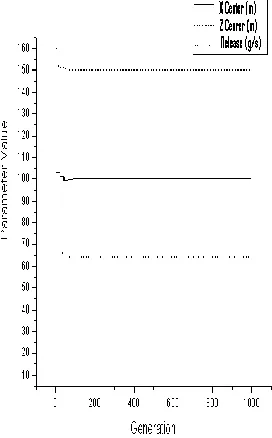
Figure 9 Convergence of Parameter Values for Experiment 1

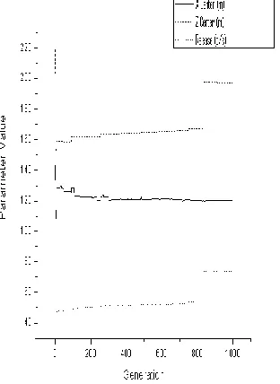
The second experiment attempted to inverse three parameters using the light wind dataset. The backwards PGA was again able to solve the dispersion equation system and accurately provide the value of the source amplification (99 g/s). Without any knowledge of this wind velocity, the PGA was able to identify the light wind data set, meaning that the PGA can choose the right model from the model pool. It can also provide the correct model id as one of the estimated parameters. The backwards PGA was also able to solve the dispersion equation system and accurately provide the values of the source amplitude well as the x (x=10) and z coordinates (z=155) where it was centered. Figure 10 shows the parameter values obtained by the PGA at each generation. The horizontal axis represents the number of generations. The vertical axis represents the values of x and z that were obtained for each generation as well as the concentration. The x and z values of the source location were able to converge within 200 generations. The initial source release had a much greater variance and needed an extra one hundred generations to converge.

Figure 10 Convergence of Parameter Values for Experiment 2

Obtaining the Parameters Using Only the Surface Layer Data

(8)

International Journal of Emerging Technology and Advanced Engineering

[image:8.612.344.539.161.351.2]

181

[image:8.612.69.255.166.402.2]

Figure 11 X Value Convergence for Experiment 3

[image:8.612.64.242.456.667.2]

Figure 12: Z Value Convergence for Experiment 3

Figure 13: PGA Generation of Source Release for Experiment 3

(9)

International Journal of Emerging Technology and Advanced Engineering

[image:9.612.338.494.138.360.2]

182

Figure 14: Convergence of Dispersion Parameter for Experiment 4

In the final experiment the PGA was able to successfully calculate the x and z coordinates as well as which model was used. An aerial view of the concentration is shown in Figure 15. The amount of the source release was found within 999 generations and using only 5 seconds of CPU time. Even though the PGA ran through 999 generations, convergence occurred quickly within 19 generations. Figure 16 displays the parameter values obtained. There was a lot more early volatility for the x and z values when compared to the previous experiment. Particularly surprising is the area between the 2nd and 7th generations where the x and z switch values.

[image:9.612.61.217.149.363.2]

Figure 15 Values obtained by the PGA in Experiment 5

A closer look at the results of the PGA model reveals the intra-generation process. First all the individual members of each generation were normalized by dividing each by the highest possible value. This makes the comparison much easier as it fixes the range between 0 and 1. Figure 16 shows the values obtained for the first generation. A great amount of noise is present and the 64 member ensemble is scattered. As the PGA runs more generations each parameter value becomes more harmonized. The best guess set of values is replicated and with mutation the next generation ensemble becomes closer to the real value. Each parameter in the graph is represented by a different shape. In Figure 17 each parameter in Generation 7 is being grouped into the correct value in certain clusters. There are still a lot of values which are incorrect thereby creating noise. By Generation 32, almost full convergence is realized as shown in Figure 18.

(10)

International Journal of Emerging Technology and Advanced Engineering

[image:10.612.68.230.141.352.2]

183

Figure 16: Values obtained for Generation 1 in Experiment 5

[image:10.612.328.508.142.382.2]

Figure 17: Values Obtained for Generation 7 in Experiment 5

[image:10.612.342.515.442.641.2]

(11)

International Journal of Emerging Technology and Advanced Engineering

184

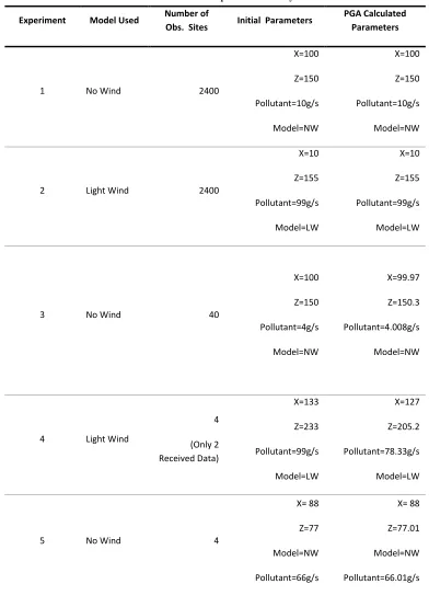
The results obtained and displayed in Table 1 indicate the backwards PGA is an effective method in obtaining the starting parameters of a single point source emission when using either the No Wind or Light Wind model.

VI. SUMMARY AND CONCLUSION

The backwards PGA was able to quickly obtain the correct parameters in Experiments 1 and 2. A great majority of the calculated parameters were an exact match from the values entered into the model or within 2%. As the number of sites decreased and the desired parameters increased, the number of generations that were needed also increased. The intra-generation convergence was shown in Experiment 5. Obtaining all four parameters from only four known concentrations in Experiment 5 is impressive. The backwards PGA was also able to successfully recognize the observation data coming from the no-wind and light-wind environment and differentiate which of the two models should be selected, as well as the release rate of the source. Although there are other models which have not been tested, the backwards PGA has proven to be an effective method for obtaining the location of the pollutant source.

Acknowledgements

This work was sponsored by the Department of Energy Samuel Massie Chair of Excellence Program under Grant No. DF-FG01-94EW11425. The views and conclusions contained herein are those of the writers and should not be interpreted as necessarily representing the official policies or endorsements, either expressed or implied, of the funding agency.

REFERENCES

[1] Agarwal, P., Yadav, A. K., Gulati, A., S., Rao, S., Singh, M. P., Nigam, S., and Reddy, N., (1995). Surface layer turbulence processes during low windspeed in tropics. Atmospheric Environment. 29, 2089-2098

[2] Allen, T., Young, S. and Haupt, S., (2007). Improving pollutant source characterization by better estimating wind direction with a genetic algorithm. Atmospheric Environment. 41, 11, 2283-2289. [3] Ayra, S.P., (1995). Modeling and parameterization of near source

diffusion in weak winds. Journal of Applied Meteorology 34. 1112-1122

[4] Charbonneau, P. and Knapp, B., (1995). A User's guide to PIKAIA 1.0, NCAR Technical Note 418+IA (Boulder: National Center for Atmospheric Research).

[5] Goldberg, D., (1989). Genetic Algorithms. Addison Wesley. [6] Metcalfe, Travis., (2001). Computational Asteroseismology,

University of Texas at Austin. Dissertation http://www.whitedwarf.org/metcalfe/index.htm

[7] Mitchel, M., (1998). An Introduction to Genetic Algorithms. MIT Press..

[8] Oettl, D., Raimund, A. and Sturm, P., (2001). A new method to estimate diffusion in stable, low-wind conditions. Journal of Applied Meteorology 40, 259-268

[9] Sagendorf, J. F., and Dickson, C. R., (1974). Diffusion under low windspeed, inversion conditions. NOAA Tech. Memo. ERL ARL-52, 89

[10] Sharan, M. and Modani, M., (2005). An analytical study for the dispersion of pollutants in a finite layer under low wind conditions. Pure and Applied Geophysics. 162, 1861-1892

[11] Sharan M., Singh M.P., and Yadav A.K., (1996). Mathematical model for atmospheric dispersion in low winds with eddy diffusivities as linear functions of downwind distance.Atmospheric Environment, 30, 7, 1137-1145

[12] Sharan M. and Yadav A.K., (1998). Simulation of diffusion experiments under light wind, stable conditions by a variable K-theory model. Atmospheric Environment, 32, 20, 3481-3492 [13] Wall, M., (2003). Introduction to Genetic Algorithms. http://

(12)

International Journal of Emerging Technology and Advanced Engineering

[image:12.612.114.506.161.715.2]

185

Table 1. Experiment Summary

Experiment Model Used Number of

Obs. Sites Initial Parameters

PGA Calculated Parameters

1 No Wind 2400

X=100

Z=150

Pollutant=10g/s

Model=NW

X=100

Z=150

Pollutant=10g/s

Model=NW

2 Light Wind 2400

X=10

Z=155

Pollutant=99g/s

Model=LW

X=10

Z=155

Pollutant=99g/s

Model=LW

3 No Wind 40

X=100

Z=150

Pollutant=4g/s

Model=NW

X=99.97

Z=150.3

Pollutant=4.008g/s

Model=NW

4 Light Wind

4

(Only 2 Received Data)

X=133

Z=233

Pollutant=99g/s

Model=LW

X=127

Z=205.2

Pollutant=78.33g/s

Model=LW

5 No Wind 4

X= 88

Z=77

Model=NW

Pollutant=66g/s

X= 88

Z=77.01

Model=NW