An aly si s of e ff e c tiv e a n d o r g a n
d o s e e s ti m a ti o n i n CT w h e n u si n g
mA m o d ul a ti o n : a si n gl e s c a n n e r
pilo t s t u d y
Too t ell, AK, S z c z e p u r a , K a n d H o g g , P
h t t p :// dx. d oi.o r g / 1 0 . 1 0 1 6 /j. r a di. 2 0 1 7 . 0 2 . 0 0 6
T i t l e
An aly si s of eff e c tiv e a n d o r g a n d o s e e s ti m a ti o n i n CT w h e n
u si n g mA m o d u l a tio n : a si n gl e s c a n n e r p ilo t s t u d y
A u t h o r s
Too t ell, AK, S z c z e p u r a , K a n d H o g g , P
Typ e
Ar ticl e
U RL
T hi s v e r si o n is a v ail a bl e a t :
h t t p :// u sir. s alfo r d . a c . u k /i d/ e p ri n t/ 4 1 4 5 6 /
P u b l i s h e d D a t e
2 0 1 7
U S IR is a d i gi t al c oll e c ti o n of t h e r e s e a r c h o u t p u t of t h e U n iv e r si ty of S alfo r d .
W h e r e c o p y ri g h t p e r m i t s , f ull t e x t m a t e r i al h el d i n t h e r e p o si t o r y is m a d e
f r e ely a v ail a bl e o nli n e a n d c a n b e r e a d , d o w nl o a d e d a n d c o pi e d fo r n o
n-c o m m e r n-ci al p r iv a t e s t u d y o r r e s e a r n-c h p u r p o s e s . Pl e a s e n-c h e n-c k t h e m a n u s n-c ri p t
fo r a n y f u r t h e r c o p y ri g h t r e s t r i c ti o n s .
Analysis of effective and organ dose estimation in CT when using mA modulation:
A single scanner pilot study
Andrew Tootell BSc(Hons), PGCert, MSc, FHEA
Abstract
Effective dose (ED) estimation in CT examinations can be obtained by combining dose length product (DLP) with published ED per DLP coefficients or performed using software. These methods do not account for tube current (mA) modulation which is influenced by patient size.
Aim
To compare different methods of organ and ED estimation to measured values when using mA modulation in CT chest, abdomen and pelvis examinations.
Method
Organ doses from CT of the chest, abdomen and pelvis were measured using digital dosimeters and a dosimetry phantom. ED was calculated. Six methods of estimating ED accounting for mA
modulation were performed using ImPACT CTDosimetry and Dose Length Product to ED coefficients. Corrections for the phantom mass were applied resulting in 12 estimation methods. Estimated organ doses from ImPACT CTDosimtery were compared to measured values.
Results
Calculated EDs were; chest 12.35 mSv (±1.48 mSv); abdomen 8.74 mSv (±1.36 mSv) and pelvis 4.68 mSv (±0.75 mSv). There was over estimation in all three anatomical regions. Correcting for phantom mass improved agreement between measured and estimated ED. Organ doses showed
overestimation of dose inside the scan range and underestimation outside the scan range. Conclusion
Introduction
Advances in technology have facilitated Computed Tomography’s (CT) expansion in providing rapid complex submillimetre imaging allowing more accurate diagnoses to be made [1-3]. In many instances CT is the first line investigation, however this has resulted in it becoming the dominant source of radiation risk/dose in medical imaging [3]. As with any medical imaging procedure
involving radiation, there is a need for all involved to be aware of and monitor dose to patients; this is achieved by dose estimation as direct measurement of organ dose is not possible in the clinical environment.
Effective dose is often calculated by combining dose length product [DLP], (the product of the CT dose index volume (CTDivol) and scan length) with published coefficients (k-coefficient) [4-7]. This approach uses data published by the American Association of Physicists in Medicine (AAPM) [4]. Critics of this method state that the use of tissue weighting factors from ICRP 60 and scanner data from as early as 1990 means that the coefficients lack relevance to modern multidetector scanners in use today [7]. Updated figures have been published and used by Elbakri and Kirkpatrick [5] and Huda et al [6]. Both these articles argued that due to the updated tissue weighting factors published by the ICRP the conversion factors require updating too. Huda et al [6] provide figures that are independent of the make and model of scanner whilst Elbakri and Kirkpatrick [5] argued that accuracy can be improved further by taking into account scanner-specific results. In Elbakri and Kirkpatrick’s paper figures for a range of scanner types are provided [5].
An alternative method of effective dose estimation can be performed by combining CTDivol with data produced using Monte Carlo mathematical simulation. Data provided by the UK’s National Radiological Protection Board (NRPB) can be used to calculate effective dose by utilising ImPACT’s CT dosimetry tool (CTDosimetry V1.0.4) [8]. Although convenient, the data used in the Monte Carlo simulation was generated from early CT systems (not multidetector) therefore effective dose estimation has to be performed by fitting the characteristics of newer scanners to older designs [9]. This has the potential to introduce error [10].
Tube current modulation (mA modulation) is not taken into account when dose estimations are performed using the software or k-coefficients. mA modulation is standard on modern CT imaging equipment and it has the ability to manipulate the exposure and therefore dose as the patient is imaged. The ability to accurately estimate dose using fixed tube current has been shown but organ dose generally decreases with the use of tube current–modulated acquisition and this should be taken into account in any estimation method, but patient size can directly affect the dose reduction achieved [11].
increase in mass for pelvis acquisitions. For fixed exposure parameters, effective dose decreases as patient mass increases suggesting that dose is likely to be overestimated [13].
This initial work utilised a single scanner type and phantom size and with a focuses on organ and effective dose calculation accuracy using mA modulation in CT of the chest, abdomen and pelvis. This paper examines different methods of dose estimation and compares these to direct
measurements of organ doses made using an anthropomorphic phantom and MOSFET dosimeters. Effective dose calculations were compared against values generated using k-coefficients and ImPACT software. To account for mA modulation mass weighted corrections were applied in an attempt to improve accuracy for effective dose calculations.
Method
For CT of the chest, abdomen and pelvis twelve methods of estimating effective dose were used (Table 1) CT dosimetry software published by the ImPACT CT scanner evaluation group (ImPACT CTDosimetry spreadsheet v 1.0.4, ImPACT, London, UK) was used to estimate organ and effective dose. For each anatomicalregion, the DLP was recorded. Dose per DLP figures published by the American Association of Physicists in Medicine (AAPM) [4], Huda et al [6] and Elbakri and Kirkpatrick [5] were used to calculate effective dose (Table 2Table 2). One method of calculating effective dose from directly measured organ doses using MOSFETs was undertaken for CT of the chest, abdomen and pelvis using MOSFET dosimeters (Best Medical Canada, Kanata, Canada) and a male ATOM dosimetry phantom model 701-D (CIRS Inc. Virginia, USA). In all cases a Toshiba Aquillion 16 Multidetector CT scanner was used (Toshiba medical systems, Otawara-Shi, Japan). This system utilises filtered back projection reconstruction and for the purpose of the data collection
manufacturer recommended reconstruction algorithms and a mA standard deviation of 5. The CT system uses Toshiba’s SUREExposure3D method of tube current modulation during exposure. This uses the anterior-posterior and lateral scan plan radiograph to ascertain the optimum exposure. The system modulates the tube current in the z-axis and during rotation [14].
Direct dose measurements (MOSFET) were taken as the gold standard against which estimation methods were compared [15, 16].
Table 1 Methods of dose estimation
1. ImPACT effective mA 2. ImPACT average mA 3. ImPACT mA modulation 4. AAPM k-coefficient 5. Huda et al k-coefficient
6. Elbakri and Kirkpatrick k-coefficient 7. Mass corrected ImPACT effective mA 8. Mass corrected ImPACT average mA 9. Mass corrected ImPACT mA modulation 10. Mass corrected AAPM k-coefficient 11. Mass corrected Huda et al k-coefficient
Table 2 Coefficients for calculation of effective dose from DLP
k-coefficient mSv/mGy.cm
AAPM [4] Huda et al [6] Elbakri and Kirkpatrick [5]
Chest 0.014 0.017 0.020
Abdomen 0.015 0.016 0.017
Pelvis 0.015 0.018 0.017
Dose measurement
MOSFET dosimeters provide an accurate and reproducible method of collecting organ dosimetry data [17]. In this work four banks of five dosimeters were used (n=20). Calibration was performed as per manufacturer instructions at a tube voltage of 120 kV using the supplied calibration jig and a calibrated RaySafe X2 with R/F sensor (Unfors RaySafe AB, Bildal, Sweden). The error of these was 2.01%.
Table 3 Table stating the number of MOSFET locations used for organ dose measurement
Organ Number of dosimeter locations
Adrenals 2
Bladder 16
Brain 11
Breast 2
Active bone Marrow 85
Clavicle 20, Cranium 4 Cervical Spine 2
Femora 4 Mandible
6 Pelvis 18 Ribs 18 Scapulao 9 Sternum 4
Thoraco-lumbar Spine 9
Gall Bladder 5
Heart 2
Intestine (Small and large) 16
Colon 11
Small intestine 5
Kidneys 16
Liver 30
Lungs 36
Oesophagus 3
Pancreas 5
Prostate 3
Spleen 14
Stomach 11
Testes 2
Thyroid 10
Thymus 4
locations in the anterior of C2 and upper oesophagus were used to calculate extra thoracic organ dose
locations in the left and right lingula of the mandible and to the left and right of the
sublingual fossa were used to calculate salivary gland organ dose ×
locations in the left and right lingula of the mandible were used to calculate oral mucosa organ dose
o
For each scan, the dose length product (DLP) and the recorded effective mAs were noted. The mean DLP was calculated. Axial images were reconstructed at 1 mm slices to match the acquisition’s collimation. The mAs values for each axial image were recorded and an average mAs was calculated (Table 4).
Table 4 Imaging parameters
Chest Abdomen Pelvis
kV 120 120 120
Auto mA standard deviation 5 5 5
Rotation time (s) 0.5 0.5 0.5
݉ܣݏ 235 235 235
݉ܣݏത 203.21 201.41 211.34
Acquired slice thickness (detector length in z-axis)
16 x 1 mm 16 x 1 mm 16 x 1 mm
Pitch 0.938 0.938 0.938
ܦܮܲത 904.49 792.72 791.76
ܥܶܦܫത 33.2 33.2 33.2
Comparison of ATOM and ImPACT standard phantoms
Figure 2 Comparison of the proportions of the chest, (left) has been scaled by a factor of 1.07
The phantom used in ImPACT’s CT dosimetry software for effective dose calculations is
phantom has a mass of 73 kg and consists of the head and torso only. Acc accounts for only 55.4 % of total
Table 4 Relative weight of body segments for an adult male
Region/limb Torso
Head and Neck Upper legs Lower legs Feet Upper arms Lower arms Hands TOTAL
Using the data, a total body mass of the
much greater at 131.8 kg; an increase in mass of 88.29% was created to calculate the correction factor for mass. relationship remained constant (
parison of the proportions of the chest, abdomen and pelvis of the two phantoms. ) has been scaled by a factor of 1.07 relative to the software phantom
The phantom used in ImPACT’s CT dosimetry software that was used in the development of is based on a whole body mass of 70 kg [5, 6, 8, 21
phantom has a mass of 73 kg and consists of the head and torso only. According to total body mass [22] (Table 5).
Relative weight of body segments for an adult male [22]
Percentage contribution to total body mass (%) 48.3
7.1 21.0 9.0 3.0 6.6 3.8 1.2 100
body mass of the ATOM phantom was calculated. The resulting increase in mass of 88.29%. Using the work of Castellano was created to calculate the correction factor for mass. An assumption was made that this relationship remained constant (R2=1).
The dosimetry phantom
was used in the development of the DLP 21]. The ATOM ording to Tozeren this
Percentage contribution to total body mass (%)
Dose calculations using ImPACT CT Dosimetry software was performed in three ways;
(i) Using the effective mAs quoted by the scanner for the full range of the acquisition, (ii) Using the average mAs for the full range of the acquisition,
(iii) Using the mAs for each axial slice and summing the organ and effective doses to give final figures.
For method 3 in Table 1 a macro was created to be used within the ImPACT Excel spreadsheet that calculated the start and finish position for each slice and the corresponding mAs to calculate the effective dose per slice, which was then summated for the whole scan. The Toshiba Aquillion 16 has an overbeaming requirement of 2 rotations (1 at each end of the scan) [23]. With a collimation of 16x1 mm and a pitch of 0.938 an additional 15.0 mm at each end of the scan is required. When scaled, this is equivalent to 16.05 mm at the start and end of the acquisition in the simulation. The mA for the first and last slices was used as the mA for the respective upper and lower overbeamed sections of the scan for the mA modulation calculation. Comparisons between mass corrected and non-corrected figures using data from Table 5Table 4 were made.
Comparison of Organ doses
[image:11.595.43.564.49.260.2]Effective dose is calculated by summing the weighted equivalent organ doses. Any difference in measured and estimated organ doses would be carried through into the final effective dose estimations. Comparison of estimated and measured organ doses was carried out to establish any sources of error. Unlike methods using DLP and conversion factors, dose estimation using ImPACT CT Dosimetry software allows figures for organ dose to be collated so this comparison could only analyse dose estimations using ImPACT CT Dosimetry software. It was also not feasible to correct for mass as accurate estimation of the distribution of intrathoracic and visceral fat was not possible. The difference between simulated and measured organ doses was calculated for each method (i. ImPACT
effective mA. ii. ImPACT average mA. iii. ImPACT mA modulation). These values were compared statistically using a single factor ANOVA.
Results
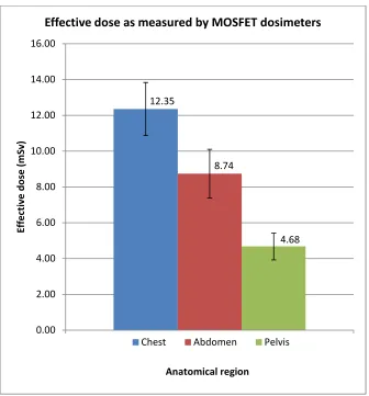
[image:12.595.72.408.215.576.2]Effective doses calculated from the MOSFET organ dose measurements (Figure 4) were 12.35 mSv (±1.48 mSv) for CT of the chest; 8.74 mSv (±1.36 mSv) for CT of the abdomen and 4.68 mSv (±0.75 mSv) for CT of the pelvis.
Figure 4 Calculated effective dose
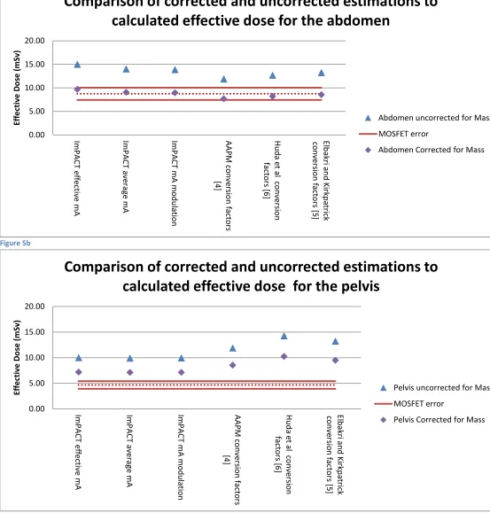
Table 6 and Figure 5 illustrate the comparison of effective dose between measured and calculated values, with and without correction of phantom mass. Figure 5 demonstrates that using mass corrected values leads to greater accuracy for the calculated effective dose in comparison to the measured values.
12.35
8.74
4.68
0.00 2.00 4.00 6.00 8.00 10.00 12.00 14.00 16.00
E
ff
e
ct
iv
e
d
o
se
(
m
S
v
)
Anatomical region
Effective dose as measured by MOSFET dosimeters
Table 5 Effective dose measurement and calculation methods.
Effective Dose (mSv)
Method Chest Abdomen Pelvis
Calculated (MOSFET) 12.35 (±1.48) 8.74 (±1.36) 4.68 (±0.75) Estimated (Uncorrected for mass)
ImPACT effective mA 19.00 15.00 10.00
ImPACT average mA 17.00 14.00 9.90
ImPACT mA modulation 17.08 13.86 9.93
AAPM conversion factors [4] 12.66 11.89 11.88
Huda et al conversion factors [6] 15.38 12.68 14.25
Elbakri and Kirkpatrick conversion factors [5] 17.91 13.24 13.22 Estimated (Corrected for mass)
Mass corrected ImPACT effective mA 12.30 9.71 7.20
Mass corrected ImPACT average mA 11.00 9.06 7.13
Mass corrected ImPACT mA modulation 11.05 8.97 7.15
Mass corrected AAPM conversion factors [4] 8.19 7.69 8.55
[image:13.595.23.571.448.717.2]Mass corrected Huda et al conversion factor [6] 9.95 8.21 10.26 Mass corrected Elbakri and Kirkpatrick conversion factors [5] 11.59 8.57 9.51
Figure 5a 0.00 5.00 10.00 15.00 20.00 Im P A C T e ff e ct iv e m A Im P A C T a ve ra g e m A Im P A C T m A m o d u la tio n A A P M c o n ve rs io n fa ct o rs [4 ] H u d a e t a l co n ve rs io n fa ct o rs [6 ] E lb a k ri a n d K ir k p a tr ic k co n ve rs io n fa ct o rs [5 ] E ff e ct iv e D o se ( m S v )
Comparison of corrected and uncorrected estimations to
calculated effective dose for the chest
Chest uncorrected for Mass
MOSFET error
Figure 5b
[image:14.595.18.578.394.667.2]Figure 5c
Figure 5 Comparison of corrected and uncorrected effective dose estimations of the (a) chest (b) abdomen and (c) pelvis to calculated effective dose
0.00 5.00 10.00 15.00 20.00 Im P A C T e ff e ct iv e m A Im P A C T a ve ra g e m A Im P A C T m A m o d u la tio n A A P M c o n ve rs io n fa ct o rs [4 ] H u d a e t a l co n ve rs io n fa ct o rs [6 ] E lb a k ri a n d K ir k p a tr ic k co n ve rs io n fa ct o rs [5 ] E ff e ct iv e D o se ( m S v )
Comparison of corrected and uncorrected estimations to
calculated effective dose for the abdomen
Abdomen uncorrected for Mass
MOSFET error
Abdomen Corrected for Mass
0.00 5.00 10.00 15.00 20.00 Im P A C T e ff e ct iv e m A Im P A C T a ve ra g e m A Im P A C T m A m o d u la tio n A A P M c o n ve rs io n fa ct o rs [4 ] H u d a e t a l co n ve rs io n fa ct o rs [6 ] E lb a k ri a n d K ir k p a tr ic k co n ve rs io n fa ct o rs [5 ] E ff e ct iv e D o se ( m S v )
Comparison of corrected and uncorrected estimations to
calculated effective dose for the pelvis
Pelvis uncorrected for Mass
MOSFET error
Table 6 Comparison of estimated organ doses using mean, effective and modulated mAs for CT of the chest, abdomen and Pelvis.
Organ dose (mGy)
Chest Abdomen Pelvis
Measured
ImPACT CTDosimetry
Measured
ImPACT CTDosimetry
Measured
ImPACT CTDosimetry
Organ ݉ܣݏത ݉ܣݏ ݉ܣݏௗ ݉ܣݏത ݉ܣݏ ݉ܣݏௗ ݉ܣݏത ݉ܣݏ ݉ܣݏௗ
Gonads 0.04 0.00 0.00 0.00 0.16 0.07 0.07 0.07 5.58 37.00 39.00 36.00
Bone Marrow 8.10 12.00 14.00 12.22 4.55 8.50 9.30 8.59 5.45 10.00 10.00 10.01
Colon 0.51 0.35 0.40 0.32 14.3 19.00 20.00 18.76 16.6 23.00 24.00 22.81
Lung 24.7 45.00 52.00 45.27 5.48 9.50 10.00 9.44 0.16 0.04 0.05 0.04
Stomach 11.3 8.80 10.00 7.87 26.0 41.00 45.00 40.78 2.02 1.00 1.10 1.04
Bladder 0.09 0.02 0.02 0.02 1.93 1.10 1.20 1.16 19.8 47.00 49.00 47.93
Breast 27.7 35.00 40.00 36.79 1.47 1.80 2.00 1.79 0.08 0.04 0.04 0.04
Liver 18.9 14.00 17.00 12.71 22.4 38.00 41.00 37.70 0.71 0.62 0.65 0.62
Oesophagus 22.7 53.00 61.00 53.35 3.02 1.40 1.60 1.43 0.07 0.01 0.01 0.01
Thyroid 16.3 8.00 9.30 8.39 0.37 0.14 0.16 0.14 0.05 0.01 0.01 0.01
Brain 0.32 0.30 0.35 0.31 0.01 0.01 0.01 0.01 0.03 0.00 0.00 0.00
Salivary Glands 2.41 0.30 0.35 0.31 0.39 0.01 0.01 0.01 0.07 0.00 0.00 0.00
Discussion
The options of mA value that are used within the ImPACT CTDosimetry software values (effective, average or modulated) has an insignificant effect on the estimated effective dose with the coefficient of variation of 6.4%, 4.4% and 0.5% for the chest, abdomen and pelvis respectively. Establishing the mAs per slice is a time consuming process and for convenience, the effective mAs can be used when estimating effective dose using ImPACT CTDosimetry software. This value is easily obtained from CT imaging equipment.
With the exception of the AAPM k-coefficient, uncorrected effective dose was over estimated (Figure 5). There was closer agreement for the CT of the chest (Figure 5a) with over estimation ranging from 2.48% to 42.4% (0.31 mSv to 6.65 mSv). There was poorer agreement in the abdomen (Figure 5b) and pelvis (Figure 5c) with over estimation of 30.54% to 52.74% (3.15 mSv to 6.26 mSv) and 72.48% to 101% (6.26 mSv to 9.57 mSv) respectively.
Tube current modulation takes into account patient size within set parameters. The phantom used in this study is larger than the phantom used within ImPACT’s software and in the development of the k-coefficients therefore effective dose should be lower [4-6, 13]. Correcting for mass improved agreement between the effective dose estimations and calculations. Differences were 40.51% to -0.41% (-4.16 mSv to 0.05 mSv) in the chest, -12.78% to 3.60% (-1.05 mSv to 0.32 mSv) in the abdomen. It can be seen from Figure 5a,b and c that the majority of the mass corrected values fall within the error of the MOSFET dosimeters indicating no significant differences between the calculated and estimated values. Effective dose for the pelvis (Figure 5c) showed the greatest disagreement after correcting for mass with differences to MOSFET ranging from 41.76% to 74.70% (2.47 mSv to 5.58 mSv). The disagreement between effective dose of the pelvis suggests that the correction factor used is requires further research utilising phantoms of different sizes.
ANOVA showed no statistical difference in the estimation of organ dose using the average, effective or modulated mA (p=0.9). Using the mean of these three methods a comparison of estimated and measured organ doses shown in Table 7 highlights a pattern. It is apparent that organs within the scan range have an average estimate that is higher than measured values and those organs outside the scan range i.e. those organs whose dose comes from scattered radiation, have estimates that are lower than the measured values. To explore the effect this would have on effective dose estimations and calculations the tissue weighting factors were applied and the percentage contribution to effective dose of organs within and outside the scan range was calculated (Table 8). It is recognised that certain organs would be part in and part out of the scan range but for the purpose of this analysis, organs that were mostly in the scan range were classified as ‘in’ and vice versa.
Table 7 Percentage contribution of organs inside and outside the scan range to effective dose calculations
Percentage contribution to calculated effective dose (%)
inside outside
Chest 71.5 28.5
Abdomen 58.5 41.5
The chest and abdomen show better balance between contributions of organs inside and outside the scan range which would explain why these estimations are in closer agreement when compared to the chest and pelvis. The pelvis, however, has an imbalance with the greatest contribution to the effective dose calculation coming from organs inside the scan range- specifically the bladder, gonads and colon. With the suggested tendency of ImPACT dosimetry software to over-estimate organ dose inside the primary beam the reason for the large difference in calculated effective dose using measured organ dose to estimated effective dose is apparent. Reasons for these errors require further investigation and should focus on the suitability of the Monte Carlo data sets used in ImPACT’s CTDosimetry software, the “best-fitting” of newer scanners to data in the ImPACT CTDosimetry software.
Limitations
It is recognised that this work is not without limitations. Only one scanner type and phantom was used. The tube current modulation parameters remained constant through the data collection and only filtered back projection reconstruction was used. Investigation into the mass correction for CT of the pelvis is required as this work has shown that over estimation occurs even after correction for mass. Should accurate organ dose estimations be required, clinicians should be aware of the under and over estimation of dose for organs inside and outside the scan range.
This work has shown that in this context, there is the potential to improve the accuracy of effective dose estimations by accounting for patient mass. Further work is required improve the accuracy of the mass correction factor of the pelvis and externally validate the factors for the chest and
abdomen. Experimentation using phantoms of different sizes, imaging parameters and CT scanners from different manufacturers is planned.
Conclusion
1. Lowe AS and Kay CL, Recent developments in CT: a review of the clinical applications and advantages of multidetector computed tomography. Imaging, 2006. 18(2): p. 62-67. 2. Golding SJ, Multi-slice computed tomography (MSCT): the dose challenge of the new
revolution. Radiation Protection Dosimetry, 2005. 114(1-3): p. 303-307.
3. Shrimpton P, Hillier MC, S M, and SJ G, Doses from Computed Tomography (CT) Examinations in the UK – 2011 Review. 2014, Public Health England: Oxfordshire.
4. American Association of Physicists in Medicine, The Measurement, Reporting, and Management of Radiation Dose in CT, in Report of AAPM Task Group 23 of the Diagnostic Imaging Council CT Commitee. 2007: Maryland, USA.
5. Elbakri IA and Kirkpatrick IDC, Dose-Length Product to Effective Dose Conversion Factors for Common Computed Tomography Examinations Based on Canadian Clinical Experience.
Canadian Association of Radiologists Journal, 2013. 64(1): p. 15-17.
6. Huda W, Ogden KM, and Khorasani MR, Converting Dose-Length Product to Effective Dose at CT. Radiology, 2008. 248(3): p. 995-1003.
7. McNitt-Gray M, Assessing Radiation Dose: How to Do It Right, in 2011 AAPM CT Dose Summit. 2011: Denver.
8. ImPACT, CT Patient Dosimetry Calculator. 2003, Medical Devices Agency: London.
9. Tootell A, Szczepura K, and Hogg P, An overview of measuring and modelling dose and risk from ionising radiation for medical exposures. Radiography, 2014. 20(4): p. 323-332. 10. Groves AM, Owen KE, Courtney HM, Yates SJ, Goldstone KE, Blake GM, et al., 16-detector
multislice CT: dosimetry estimation by TLD measurement compared with Monte Carlo simulation. Br J Radiol, 2004. 77(920): p. 662-5.
11. Angel E, Yaghmai N, Jude CM, DeMarco JJ, Cagnon CH, Goldin JG, et al., Dose to
Radiosensitive Organs During Routine Chest CT: Effects of Tube Current Modulation. AJR. American journal of roentgenology, 2009. 193(5): p. 1340-1345.
12. McCollough CH, Leng S, Yu L, Cody DD, Boone JM, and McNitt-Gray MF, CT Dose Index and Patient Dose: They Are Not the Same Thing. Radiology, 2011. 259(2): p. 311-316.
13. Castellano E, CT Dose calculations for individual patients - what you should know, in 12th CT Users Group. 2010: London.
14. Centre for Evidence-based Purchasing (CEP), Comparative Specifications 16 slice CT scanners. March 2009: NHS/PASA, London.
15. Hintenlang D, TH-C-301-03: Utilization of MOSFET Dosimeters for Clinical Measurements in Radiology. Medical Physics, 2011. 38(6): p. 3861-3861.
16. Chida K, Inaba Y, Masuyama H, Yanagawa I, Mori I, Saito H, et al., Evaluating the performance of a MOSFET dosimeter at diagnostic X-ray energies for interventional radiology. Radiological Physics and Technology, 2009. 2(1): p. 58-61.
17. D H, The Utilization of MOSFET Dosimeters for Clinical Measurements in Radiology, in Joint Programme The American Association of Physicists in Medicine (AAPM) and the Canadian Organization of Medical Physicists (COMP). 2011: British Columbia.
18. CIRS Tissue Simulation and Phantom Technology, Adult Male Phantom Model Number 701-D Appendix 5. 2010, CIRS, Inc: Virginia, USA.
19. CIRS Tissue Simulation and Phantom Technology. Dosimetry Verification Phantoms Model 701-706 Data Sheet. 2012 [cited 2012 19th January]; Available from:
http://www.cirsinc.com/file/Products/701_706/701_706_DS.pdf.
20. ICRP, The 2007 Recommendations of the ICRP, in ICRP Publication 103. 2007, Ann. ICRP. p. 2-4.
21. Huda W, Sterzik A, Tipnis S, and Schoepf UJ, Organ doses to adult patients for chest CT.
Medical Physics, 2010. 37(2): p. 842-847.
22. Tozeren A, Human Body Dynamics. 2014, New York: Springer.