An Iterative method for Solving the Container Crane Constrained Optimal Control Problem Using Chebyshev Polynomials

(1)

International Journal of Emerging Technology and Advanced Engineering

Website: www.ijetae.com (ISSN 2250-2459, ISO 9001:2008 Certified Journal, Volume 5, Issue 1, January 2015)

344

An Iterative method for Solving the Container Crane

Constrained Optimal Control Problem Using Chebyshev

Polynomials

Hussein Jaddu

1

, Amjad Majdalawi

2

1,2_{Electronics Engineering Department, Faculty of Engineering, Al Quds University, Jerusalem, Palestine}

Abstract— In this paper, a computational method for solving constrained nonlinear optimal control problems is presented with an application to the container crane. The method is based on Banks' et al. iterative approach, in which the nonlinear system state equations are replaced by a sequence of time-varying linear systems. Therefore, The constrained nonlinear optimal control problem can be converted into sequence of constrained time varying linear quadratic optimal control problems. Combining this iterative approach with parameterization of the state variables using Chebyshev polynomials will result in converting the hard constrained nonlinear optimal control problem into sequence of quadratic programming problems. To show the performance and the behavior of this method compared with other known approaches, we apply it on a practical problem namely the container crane problem and the simulation results are presented and compared with other methods.

Keywords—Banks' Iterative Technique, Chebyshev polynomials, Constrainednonlinear quadratic optimal control problem, Container Crane, State parameterization.

I. INTRODUCTION

One of the widely used methods to solve the constrained nonlinear optimal control problems is the direct method, which is based on replacing the original problem by a finite dimension mathematical programming problem [1-7]. The direct methods are implemented using the discretization or the parameterization methods or both. In its turn, the nonlinear mathematical programming problem can then be solved using different methods. One of the popular methods that are used to handle the nonlinear mathematical programming problem is the sequential quadratic programming method [8] which replaces the nonlinear mathematical programming problem by a sequence of quadratic programming problems.

Jaddu [9-11] proposed a method that is based on state parameterization via Chebyshev polynomials combined with quasilinearization to handle the constrained nonlinear quadratic optimal control problems and to convert the constrained nonlinear optimal control problem into sequence of quadratic programming problems.

Also recently Jaddu and Majdalawi [12, 13] proposed new method to solve the nonlinear optimal control problem that is based on Banks' et al [14-18] iterative technique along with the state parameterization using Chebyshev and Legendre polynomials. This iterative method is based on replacing the nonlinear dynamic state equation into sequence of linear time- varying state equations. Therefore, the nonlinear optimal control problem is replaced by sequence of time- varying linear quadratic optimal control problems.

In this paper we extend our work in [12, 13] to handle nonlinear optimal control problems subject to terminal state constraints, state variables and control variables saturation constraints. After applying the iterative technique the resulted time-varying linear optimal control problems are converted into quadratic programming problem by parameterizing the state variables via Chebyshev polynomials.

In addition, the proposed method is tested by applying it to difficult constrained nonlinear optimal control problem., namely the container crane problem to minimize the swing angle during the transfer of a container from a ship to a truck. The results of the method are compared with other results obtained using other methods.

II. PROBLEM STATEMENT

The optimal control problem treated in this paper can be stated as follows: Find an optimal controller that minimizes the following performance index

(1)

subject to the following constraints: Nonlinear dynamic system state equations and initial conditions

(2)

and terminal state constraints

(3)

(2)

International Journal of Emerging Technology and Advanced Engineering

345

(4)

Where is an positive semidefinite matrix, is an positive definite matrix, is the state vector, is the control input vector, is the initial condition vector, is matrix,

and are constant vectors of appropriate dimension, is the fixed final time and is a known final state vector . We will assume that:

The constrained nonlinear optimal control problem (1)-(4) is solved by applying iterative method to converting it into a sequence of constrained time-varying linear quadratic optimal control problems. Then, each of these problems is solved by transforming it into quadratic programming problem by using state parameterization via Chebyshev polynomials.

III. ITERATIVE TECHNIQUE

This technique was developed by Banks et al. [14-18]. In this technique, the constrained nonlinear optimal control problem (1)-(4) can be transformed into an equivalent sequence of constrained time-varying linear quadratic problems.

Applying the iterative technique to the optimal control problem described in (1)-(4), the following sequence of constrained time-varying linear quadratic optimal control problems can replace the original problem in (1)-(4): and for

Minimizes

(5)

subject to the linearized state equations and initial conditions

(6)

and to the following terminal constraints

(7)

and to the following state and control saturation constraints

(8)

where

IV. PROBLEM REFORMULATION

To convert each of the constrained time-varying linear optimal control problems (5)-(8) into a quadratic programming problem, some state variables are approximated by a finite length Chebyshev series with unknown parameters [9]. Then, the remaining state and control variables are determined as a function of the unknown parameters of the approximated state variables from the state equations (6). These approximations are used to approximate the remaining constraints, namely, initial conditions, terminal state constraints and state and control saturation constraints. For details of the state parameterization the reader is advised to consult [9].

Chebyshev polynomials are defined on the interval . Therefore, it is necessary to transform the time

interval of the original problem into .

This can be done by

(9)

Therefore, each of the constrained time-varying linear optimal control problems (5)-(8) can be reformulated and rewritten in terms of as follows:

For

Minimize

(10)

subject to:

(11)

(12)

(13)

where

V. STATE PARAMETERIZATION VIA CHEBYSHEV

POLYNOMIALS

(3)

International Journal of Emerging Technology and Advanced Engineering

346

A) System State Equations Approximation:

The state parameterization technique is implemented according to the work of [9], in which the state variables are approximated as

(14)

Where N is the length of the Chebyshev series, aiare the unknown parameters and Ti is a first type Chebyshev polynomial of order i. The control variables are obtained from the system state equations (11) as a function of the unknown parameters of the state variables. These control variables can be rewritten in terms of a finite length series of Chebyshev polynomials with unknown parameters as follows:

(15)

Where the unknown parameters are function of

unknown parameters of the state variables.

To obtain the control variables in terms of Chebyshev polynomials, it is necessary to parameterize the derivative of the state variables. This can be done using Chebyshev polynomials properties as follows [19]:

(16)

Where

(17)

B) Time-Varying Matrices and

Approximation:

The system state equations (11) shows that the two

matrices and are a function of ,

therefore it is necessary to express every dependant element in both matrices in terms of a Chebyshev series of known parameters. To this end, let

be the element of the matrix where

is the nominal trajectory of the previous iteration. Then the term can be expressed in terms of a

Chebyshev polynomials of known parameters of the form [19]:

(18)

Where

(19)

and and . The same

approximation can be done to the matrix .

C) Initial and Terminal State Constraints Approximation:

Using the Chebyshev polynomials initial value property [19], the initial condition vector is approximated as follows

(20)

The same procedure can be applied to approximate the terminal state vector at , the following approximation of the terminal state vector can be obtained

(21)

D) Control and State Saturation Constraints

Approximation:

To deal with the saturation constraints on the state and control variables we can add a slack variable to the inequality constraint to convert them into equality constraints. This method was used in [7]. However, using this method would result in two drawbacks: The first is adding a slack variable would convert the linear problem into a nonlinear one, while the second drawback is the increase in the number of the unknown parameters.

Another method to deal with the saturation constraints [20, 21] is to discretize the time interval with

discrete points, and satisfy the constraints at each point. By this, every continuous constraint is replaced by

finite dimension constraints. In this work we will apply this approach

The time interval is discretized as follows

(22)

Therefore, each of the continuous control saturation constraints is replaced by finite dimension inequality constraints. The control saturation constraints are given by

(4)

International Journal of Emerging Technology and Advanced Engineering

347

(24)

and the state saturation constraints are given by

(25)

(26)

where .

E) Performance Index Approximation:

The last step is to approximate the performance index in (10). The state and the control variables approximation in (14) and (15) can be rewritten in matrix form as

(27)

Substituting (27) into (10) , gives

(28)

Where is the approximated value of at iteration .

By letting and and noting that

both matrices and are symmetrical, Jaddu [9] derived an explicit formula for the approximated performance index, therefore can beexpressed as

(29)

Where

(30)

(31)

Where and

, are the elements of the symmetrical matrices

and respectively.

The performance index in (29) can be rewritten as follows

(32)

Where

is the

unknown parameter vector and is appositive definite [9] Hessian matrix given by

(33)

where and .

each of the time varying optimal control problems (10)-(13) is converted into quadratic programming problem as follows

(34)

subject to

(35)

(36)

Where the equality constraints are due to initial conditions (20), terminal state constraints (21), and in some cases due to unsatisfied state equations. While the inequality constraints are due to saturation constraints of the control and/or the state variables (23)-(26). After solving this standard quadratic programming problem the resulted state variables and the control variables are used in the new iteration.

VI. CONTAINER CRANE PROBLEM

In this section, we will apply the proposed method of this research to a practical and complex problem; the container crane. It is desired to transfer containers at the port of Kobe [22] from a ship to a cargo truck. For safety reasons, the objective is to minimize the swing during and at the end of the transfer operation.

Without going into the complex modeling aspects of this problem, which can be found in details in [22], this problem can be state as follows:

Find an optimal controller that minimizes the following performance index

(37)

subject to the following state equations

(38) (39) (40) (41) (42) (43)

where

(5)

International Journal of Emerging Technology and Advanced Engineering

348

(45)

and

(46) (47)

with continuous state inequality constraints

(48) (49)

Applying the iterative technique of section III and changing the time into , we get

For

Minimize

(50)

subject to the following state equations

(51)

(52)

(53)

(54)

(55)

(56)

where

(57) (58)

and

(59)

(60)

with continuous state inequality constraints

(61)

(62)

This problem was treated by Sakawa and Shindo [22], but no optimal value was reported. Goh and Teo [23] used a piecewise constant functions to parameterize the control variables and was found to be . They also used a piecewise linear functions to parameterize the control variables and found . Jaddu [11] solved this problem using the second method of quasilinearization and state parameterization using Chebyshev polynomials, and was found to be after three iterations.

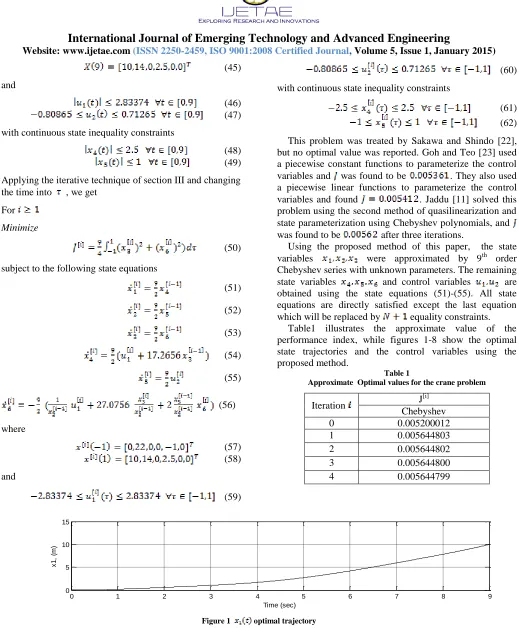
Using the proposed method of this paper, the state variables were approximated by 9th order Chebyshev series with unknown parameters. The remaining state variables and control variables are obtained using the state equations (51)-(55). All state equations are directly satisfied except the last equation which will be replaced by equality constraints.

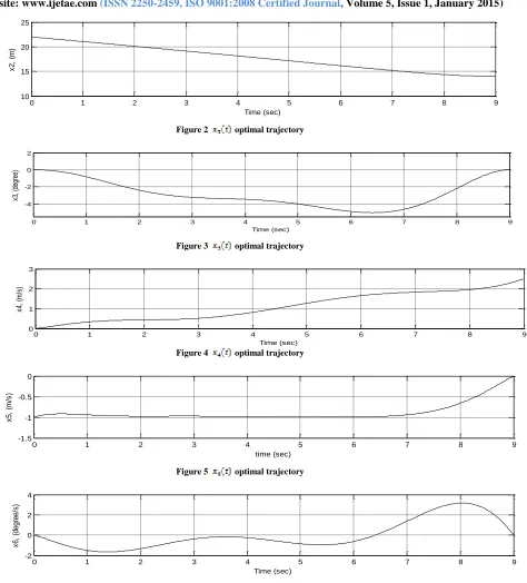
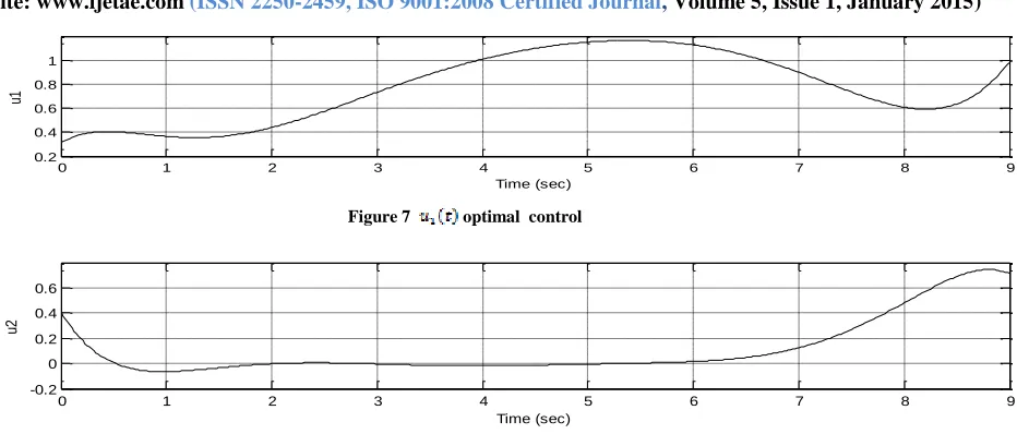
Table1 illustrates the approximate value of the performance index, while figures 1-8 show the optimal state trajectories and the control variables using the proposed method.

Table 1

Approximate Optimal values for the crane problem

Iteration J

[i]

Chebyshev

0 0.005200012

1 0.005644803

2 0.005644802

3 0.005644800

4 0.005644799

0 1 2 3 4 5 6 7 8 9

0 5 10 15

Time (sec)

x

1

,

(m

[image:5.612.47.566.74.712.2]

)

(6)

International Journal of Emerging Technology and Advanced Engineering

349

0 1 2 3 4 5 6 7 8 9

10 15 20 25

Time (sec)

x

2

,

(m

)

Figure 2 optimal trajectory

0 1 2 3 4 5 6 7 8 9

-4 -2 0 2

Time (sec)

x3

, (

de

gr

ee

)

0 1 2 3 4 5 6 7 8 9

0 1 2 3

Time (sec)

x4

,

(m

/s

)

0 1 2 3 4 5 6 7 8 9

-1.5 -1 -0.5 0

time (sec)

x

5

,

(m

/s

)

0 1 2 3 4 5 6 7 8 9

-2 0 2 4

Time (sec)

x

6

,

(d

e

g

re

e

/s

[image:6.612.90.564.122.646.2]

)

(7)

International Journal of Emerging Technology and Advanced Engineering

350

0 1 2 3 4 5 6 7 8 9

0.2 0.4 0.6 0.8 1

Time (sec)

[image:7.612.93.559.124.323.2]

u1

Figure 7 optimal control

0 1 2 3 4 5 6 7 8 9

-0.2 0 0.2 0.4 0.6

Time (sec)

u2

Figure 8 optimal control

VII. CONCLUSION

A numerical method for solving the constrained nonlinear optimal control problems is presented. This method is based using an iterative technique and the state parameterization to replace the problem by sequence of quadratic programming problems. The method is applied on the container crane optimal control problem and the simulation results show that the method give comparable results compared with other methods reported in the literature.

REFERENCES

[1] Buskens, C., Maurer, H., "SQP-method for solving optimal control problems with control and state constraints: adjoint variables, sensitivity analysis and real time control", Journal of Computational and Applied Mathematics, 120, 85–108, 2000.

[2] Betts, J. T., Practical Methods for Optimal Control using Nonlinear Programming. SIAM: Philadelphia, 2001.

[3] Goh, C. J., Teo, K. L.," Control parameterization: a unified approach to optimal control problems with general constraints.", Automatica, 24, 3-18, 1988.

[4] Jaddu, H., Shimemura, E., " Computational method based on state parameterization for solving constrained nonlinear optimal control problems", International Journal of Systems Science, 30, 275–282, 1999.

[5] Stryk, O., Bulirsch, R., " Direct and indirect methods for trajectory optimization", Annals of Operations Research,37, 357–373, 1992. [6] Troch, I., Breitenecker, F., Graeff, M., " Computing optimal

controls for systems with state and control constraints", Proceedings of the IFAC Control Applications of Nonlinear Programming and Optimization, Paris, 67–72, 1989.

[7] Vlassenbroeck, J., " A Chebyshev polynomial method for optimal

control with state constraints", Automatica, 24, 499–506, 1988.

[8] Betts, J., "Issues in the direct transcription of optimal control problem to sparse non-linear programs", Computational Optimal Control, Ed: R. Bulirsch and D. Kraft, Birkhauser, Germany, pp. 3-17, 1994.

[9] Jaddu, H., Numerical methods for solving optimal control problems

using Chebyshev polynomials, PHD Thesis, 1998.

[10] Jaddu, H., "Direct solution of nonlinear optimal control problems using quasilinearization and Chebyshev polynomials", Journal of the Franklin Institute, 339, 479-498, 2002.

[11] Jaddu, H., Vlach, M., "Successive approximation method for

non-linear optimal control problems with applications to a container crane problem", Optimal Control Applications and Methods, 23, 275-288, 2002.

[12] Jaddu, H., Majdalawi, M., " An Iterative Technique for Solving A Class of Nonlinear Quadratic Optimal Control Problems Using Chebyshev Polynomials", International Journal of Intelligent Systems and Applications(IJISA), 6, 53-57, 2014.

[13] Jaddu, H., Majdalawi, M., "Legendre Polynomials Iterative

Technique for Solving a Class of Nonlinear Optimal Control Problems", International Journal of Control and Automation, 7, 17-28, 2014.

[14] Tomas-Rodriguez, M., Banks, S. P., " Linear approximations to nonlinear dynamical systems with applications to stability and spectral theory", IMA Journal of Control and Information, 20, 1-15, 2003.

[15] Banks, S.P., Dinesh, K., "Approximate optimal control and stability of nonlinear finite and infinite-dimensional systems", Annals of Operations Research., 98, 19-44, 2000.

[16] Tomas-Rodriguez, M., Banks, S. P., "An iterative approach to eigenvalue assignment for nonlinear systems", Proceedings of the 45th IEEE Conference on Decision & Control, 1-6, 2006.

[17] Hernandez, N. C., Banks, S. P., Aldeen, M., " Observer Design for

(8)

International Journal of Emerging Technology and Advanced Engineering

351

[18] Tomas-Rodriguez, M., Banks S. P., Salamci, M. U., "Sliding Mode

Control for Nonlinear Systems: An Iterative Approach", Proceedings of the 45th IEEE Conference on Decision & Control, 1-6, 2006.

[19] Fox L and Parker I B. Chebyshev Polynomials in Numerical

Analysis, Oxford University Press, England, 1968.

[20] Neuman C. P. and A. Sen, A suboptimal control algorithm for

constrained problems using cubic splines, Automatica, 9, 601-613, 1973.

[21] Fegley, K., S. Blum, S., Bergholm, J., Calise, A., Marowitz, J.,

Porcelli, G., Sinha, L., Stochastic and deterministic design and control via linear and quadratic programming, IEEE Trans. Automatic Control, 16, 759-766, 1971.

[22] Sakawa, Y., Shindo, Y., Optimal control of container cranes,

Automatica, 18, 257-266, 1982.

[23] Teo K., C. Goh and K. Wong, A Unified Computational Approach to