Identification and quantification of transient structure borne sound sources in electrical steering systems

IDENTIFICATION AND QUANTIFICATION

OF TRANSIENT STRUCTURE-BORNE

SOUND SOURCES WITHIN

ELECTRICAL STEERING SYSTEMS

Michael STURM

IDENTIFICATION AND QUANTIFICATION

OF TRANSIENT STRUCTURE-BORNE

SOUND SOURCES WITHIN

ELECTRICAL STEERING SYSTEMS

Michael STURM

Acoustics Research Centre

School of Computing, Science and Engineering

University of Salford, Salford, UK

Contents

LIST OF FIGURES ... V

ACKNOWLEDGEMENTS ... XXII

NOMENCLATURE... XXIII

ABSTRACT ... XXX

1. INTRODUCTION ... 1

1.1. BACKGROUND... 2

1.2. THE GENERAL APPROACH OF VIRTUAL ACOUSTIC PROTOTYPING... 4

1.3. ON THE GENERATION AND ASSESSMENT OF STEERING INDUCED SOUND... 7

1.4. THE PHYSICAL PROBLEM... 8

1.5. TIME DOMAIN REPRESENTATION OF ELECTRICAL STEERING SYSTEMS... 11

1.6. THESIS OBJECTIVES... 13

2. LITERATURE REVIEW AND THEORY... 16

2.1. INTRODUCTION... 17

2.2. ASSUMPTION OF LINEAR AND TIME-INVARIANT SYSTEM BEHAVIOUR... 19

2.3. CHARACTERISATION OF STRUCTURE-BORNE SOUND SOURCES... 21

2.3.1. Mechanical mobility and related frequency response functions ... 28

2.3.2. Direct measurement of free velocity and blocked force... 31

2.3.3. Measurement of operational contact force ... 33

2.3.4. The in-situ blocked force approach ... 35

2.4. INVERSE FORCE IDENTIFICATION... 38

2.4.1. Frequency domain inverse methods and related approaches... 46

2.4.2. Direct deconvolution methods in time domain... 48

2.4.3. Time domain modal filtering ... 49

2.4.4. Inverse filtering using state-space methods... 53

2.4.5. Kalman filtering... 60

2.4.6. Sensitivity methods ... 66

2.5. SUMMARY AND CONCLUDING REMARKS... 68

3. IDENTIFICATION OF INTERNAL SOURCE LOCATIONS ... 72

3.1. INTRODUCTION... 73

3.2. ELECTRIC POWER STEERING SYSTEMS... 73

3.2.1. The functional principle... 75

3.3. SOUND PHENOMENA INDUCED BY ELECTRICAL STEERING SYSTEMS... 78

3.3.1. Functional steering sound... 78

3.3.2. Interfering steering sound... 80

3.3.3. Contact noise ... 81

Stick-slip phenomenon ... 81

Impact phenomenon ... 84

3.3.4. Relevance ranking of steering induced (transient) sounds ... 88

3.4. THE CONCEPTUAL SOURCE-PATH-RECEIVER MODEL... 91

3.4.1. The concept... 91

3.4.2. Sub-structuring into active and passive parts ... 92

3.4.3. The source-path-receiver model ... 95

3.4.4. Discussion... 96

3.5. SUMMARY... 98

4. FORCE RECONSTRUCTION IN TIME DOMAIN USING AN ADAPTIVE ALGORITHM ... 100

4.1. INTRODUCTION... 101

4.2. FUNDAMENTALS OF THE TIME DOMAIN INVERSE ROUTINE... 102

4.2.1. The conventional Least Mean Square algorithm... 102

4.2.2. Adaptive algorithm for the reconstruction of forces in time domain ... 105

4.2.3. The iterative adaptive process ... 109

4.2.4. Demonstration of the inversion routine for an ideal numerical model... 113

4.3. THE MODELLING APPROACH... 118

4.3.1. System and noise model ... 119

4.3.2. Performance evaluation ... 121

4.4. FORCE RECONSTRUCTION FOR SINGLE INPUT SINGLE OUTPUT SYSTEMS... 125

4.4.1. Application to noise free system ... 126

4.4.3. Sensitivity to errors in the system model... 130

4.4.4. Conclusions ... 132

4.5. FORCE RECONSTRUCTION FOR SINGLE INPUT MULTIPLE OUTPUT SYSTEMS... 134

4.5.1. The concept of over-determination and the averaged error gradient... 134

4.5.2. Application to noise free system ... 138

4.5.3. Sensitivity to noise in the structural responses... 142

4.5.4. Sensitivity to errors in the system model... 146

4.5.5. Conclusions ... 149

4.6. FORCE RECONSTRUCTION FOR MULTIPLE INPUT MULTIPLE OUTPUT SYSTEMS... 153

4.6.1. The generalisation of the method ... 153

4.6.2. Application to noise free system ... 157

4.6.3. Sensitivity to noise in the structural responses... 162

4.6.4. Sensitivity to errors in the system model... 165

4.6.5. Conclusions ... 172

4.7. SUMMARY AND CONCLUDING REMARKS... 176

5. CHARACTERISATION OF STRUCTURE-BORNE SOUND SOURCES IN ELECTRICAL STEERING SYSTEMS... 180

5.1. INTRODUCTION... 181

5.2. THE TEST BENCH MEASUREMENT APPROACH... 182

5.2.1. The test bench ... 183

5.2.2. State-of-the-art analysis ... 185

5.2.3. Operation and testing conditions ... 187

5.2.4. Conclusions ... 188

5.3. OBTAINING SUITABLE SYSTEM MODELS... 189

5.3.1. Measurement of (in-situ) frequency response functions ... 189

5.3.2. Data evaluation criteria based on reciprocity principle ... 193

5.3.3. Data evaluation criteria based on conductance of the mobility matrix ... 195

5.3.4. Impulse response functions from transformation ... 204

5.3.5. Conclusions ... 207

5.4. CHARACTERISATION USING ARTIFICIAL EXCITATIONS... 208

5.4.1. Experimental set-up... 209

5.4.2. Steering system with single internal source: Numerical examples ... 210

5.4.4. Steering system with multiple internal sources: Numerical example... 217

5.4.5. Steering system with multiple internal sources: Experimental example ... 220

5.4.6. Characterisation of the internal sources using test bench excitation ... 223

5.4.7. Conclusions ... 230

5.5. CORRECTION STRATEGIES FOR TEST BENCH MEASUREMENTS... 231

5.5.1. Limitations of test bench approach... 232

5.5.2. Strategy I: Correction of the measured operational responses ... 235

5.5.3. Strategy II: Reconstruction of an expanded set of input forces... 237

5.5.4. Conclusions ... 241

5.6. SUMMARY AND CONCLUDING REMARKS... 242

6. CONCLUDING REMARKS AND FUTURE WORK ... 245

REFERENCES ... 256

A APPENDICES... 273

A.1 OVERVIEW OF TIME DOMAIN INVERSE FORCE IDENTIFICATION METHODS... 273

A.2 ADDITIONAL RESULTS:INVERSE FORCE IDENTIFICATION IN TIME DOMAIN... 277

List of Figures

Figure 1.1: The physical problem behind steering induced noise in vehicles ... 9 Figure 2.1: Two-stage measurement approach for determination of contact forces in-situ. Assembled structure C comprising the source A which is active due to some internal source mechanisms sk and the passive receiver B; a,b and c represent all degree of freedom on the

corresponding interfaces of structures A, B and C, respectively; o indicates that operational measurements are conducted. ... 34 Figure 2.2: Two-stage measurement approach for determination of blocked forces in-situ. Assembled structure C comprising the source A which is active due to some internal source mechanisms sk and the passive receiver B; a,b and c represent all degree of freedom on the

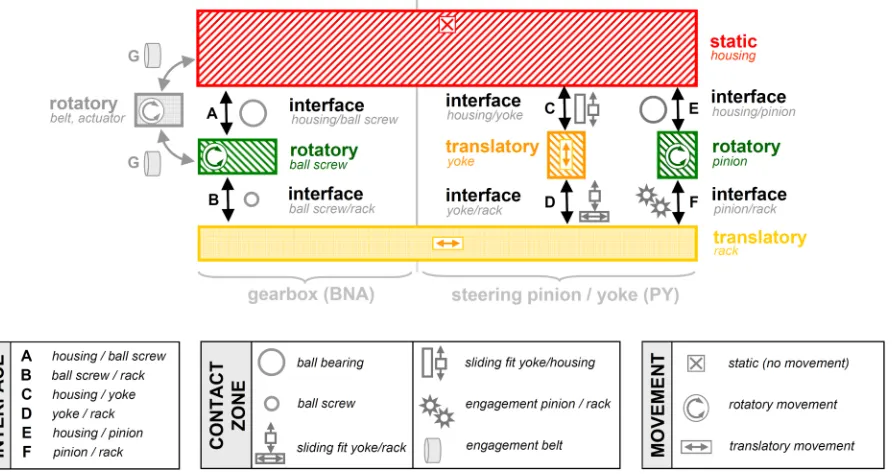
Figure 3.7. Groaning in EPS systems: Impulsive structural response (measured on the steering housing) resulting from stick-slip between bearing ring and housing while alternating left-right-steering is performed. ... 84 Figure 3.8. Impact phenomenon: (a) Exemplary model of driving mechanism forcing two neighbouring ‘inactive’ objects to vibrate; (b) Contact model descriptive for the duration of the impact between ‘active’ components... 86 Figure 3.9. Classification of sound phenomena in electric powered steering systems (EPS).. 88 Figure 3.10. Domains and components of the EPSapa PL2 steering system. ... 93 Figure 3.11. Layers within gearbox and pinion/yoke domain of EPSapa PL2 steering system

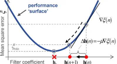
... 93 Figure 3.12. Source-path-receiver model of the EPSapa PL2 steering system. ... 96 Figure 4.1. Block diagram of adaptive system modelling (a) and detailed structure of the adaptive filter (b) ... 103 Figure 4.2. Schematic of the steepest descent rule applied to the performance surface of a single-tap transversal filter with optimum value h0... 104

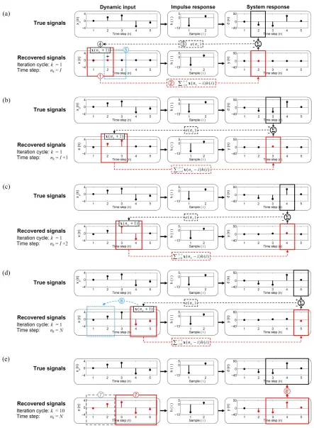
Figure 4.3. Block diagram for adaptive input reconstruction (Apostrophes indicate constrained conditions) ... 106 Figure 4.4. SISO system - force excited beam: Schematic of physical input identification problem (a), principle of cyclic iterative process achieved by consideration of additional constraints (b) and corresponding block diagram of adaptive input reconstruction algorithm (c). (Apostrophes indicate constrained conditions.) ... 109 Figure 4.5. Elementary numerical model to illustrate the iterative recursive process involved in the time domain inverse routine. Steps (a)-(d) are to be processed at each time step nk while

Figure 4.7. Simulation results for 3 different input force signatures (periodic - Simulation 1, constructed impulse sequence – Simulation 2, single transient –Simulation 3): Original and reconstructed force time history in full length (a) and close up (d), desired and reconstructed acceleration time history (b), progression of relative mean prediction error (c). ── original signal, ---- reconstructed signal using η = 0.1 % as interruption criterion, ── reconstructed signal using η = 0.001 % ... 116 Figure 4.8. Modelling approach to account for measurement noise in different data sets ... 121 Figure 4.9. Strategy invoked for identification of dynamic input forces using the time domain inverse method (TDM) and the standard frequency domain inverse method (FDM). Both methods rely on the same data sets... 123 Figure 4.10. Numerical result for noise free SISO system. Representation of signals in time domain (a, d, g, j), representation of signals in frequency domain (b, e, h,) and different estimation errors (c, f, i): ▬▬ true signal; ── reconstructed response using TDM; ─ ─

reconstructed force using TDM; ── identified force using FDM. ... 127 Figure 4.11. Numerical result for SISO system with 10% noise added to the acceleration response. Representation of signals in time domain (a, d, g, j), representation of signals in frequency domain (b, e, h,) and different estimation errors (c, f, i): ▬▬ true signal; ──

reconstructed response using TDM; ── reconstructed force using TDM; ── identified force using FDM... 128 Figure 4.12. Numerical result for SISO system with 10% noise added to the impulse response function. Representation of signals in time domain (a, d, g, j), representation of signals in frequency domain (b, e, h,) and different estimation errors (c, f, i): ▬▬ true signal; ──

constrained conditions; angle brackets denote the averaged error gradient used to update the estimated force at each time step.) ... 135 Table 4.3. Time domain inversion routine for identification of forces in single input multiple output systems. ... 137 Figure 4.14. Numerical result for noise free SIMO system. Representation of signals in time domain (a, d, g, j), representation of signals in frequency domain (b, e, h,) and different estimation errors (c, f, i): Quantities indicated by∇ξm are obtained by the SISO recursion from Table 4.1 whereas ∇ξ indicates that the SIMO recursion from Table 4.3 is used. ... 140 Table 4.4. Summary of simulation results achieved with the expanded time domain inversion routine and the standard frequency domain inverse method for the noise free SIMO system.

... 141 Figure 4.15. Comparison of the time domain inverse method (TDM) with the standard frequency domain inverse method (FDM) for the noise free SIMO system. Reconstructed force time history (left) and spectral estimation error in the identified force (right): ▬▬ true signal; ── reconstructed force using the SIMO TDM; ── identified force using the FDM.

... 142 Figure 4.16. Numerical result for SIMO system with 10% noise added to the acceleration responses. Representation of signals in time domain (a, d, g, j), representation of signals in frequency domain (b, e, h,) and different estimation errors (c, f, i): Quantities indicated by∇ξm are obtained by the SISO recursion from Table 4.1 whereas ∇ξ indicates that the SIMO recursion from Table 4.3 is used... 143 Figure 4.17. Evolution of the expanded relative mean prediction error (E-RMPE) as a function of noise added to all responses of the investigated SIMO system. The residual E-RMPE value after convergence is dependent on the noise level. ... 144 Figure 4.18. Comparison of the time domain inverse method (TDM) with the standard frequency domain inverse method (FDM) for SIMO system with 10% noise added to the responses. Reconstructed force time history (left) and spectral estimation error in the identified force (right): ▬▬ true signal; ── reconstructed force using the SIMO TDM; ──

frequency domain (b, e, h,) and different estimation errors (c, f, i): Quantities indicated by∇ξm are obtained by the SISO recursion from Table 4.1 whereas ∇ξ indicates that the SIMO recursion from Table 4.3 is used... 147 Figure 4.20. Comparison of the time domain inverse method (TDM) with the standard frequency domain inverse method (FDM) for SIMO system with 10% noise added to system model. Reconstructed force time history (left) and spectral estimation error in the identified force (right): ▬▬ true signal; ── reconstructed force using the SIMO TDM; ── identified force using the FDM... 149 Table 4.5. Summary of simulation results achieved with the expanded time domain inversion routine and the standard frequency domain inverse method for SIMO system with 5 % defective data. ... 151 Table 4.6. Summary of simulation results achieved with the expanded time domain inversion routine and the standard frequency domain inverse method for SIMO system with 10 % defective data. ... 151 Table 4.7. Summary of simulation results achieved with the expanded time domain inversion routine and the standard frequency domain inverse method for SIMO system with 25 % defective response data. ... 151 Figure 4.21. Principle of the generalised time domain inversion routine for multiple input multiple output (MIMO) systems: Schematic of force excited beam (a) corresponding cascaded block diagram for adaptive input reconstruction consisting of M MISO systems (b) and detailed schematic of one MISO block (c). (Apostrophes indicate constrained conditions; angle brackets denote the averaged error gradient; hm: (i) denotes the set of impulse response

functions between all force input locations s = [1, 2, …, S] and a single response position m.) ... 154 Table 4.8. Time domain inversion routine for identification of forces in multiple input multiple output systems. ... 156 Figure 4.22. Housing of EPSapa PL2 steering gear with assumed sources (Su) and response

positions (Pm)... 157

(c,e); spectral estimation error in reconstructed responses (f) and identified forces (g): ▬▬

true signal; ── reconstructed signal using TDM. Relative mean prediction error (E-RMPE) as performance measure of the adaptive inversion routine (h). ... 159 Figure 4.24. Comparison of the generalised time domain inverse method (TDM) with the standard frequency domain inverse method (FDM) for the noise free (2x9) MIMO system. Time signatures of reconstructed forces (a,c) and spectral estimation error in the identified force (b,d): ▬▬ true signal; ── reconstructed force using the MIMO TDM; ── identified force using the FDM... 161 Table 4.10. Summary of simulation results achieved with the generalised time domain inversion routine and the standard frequency domain inverse method for all investigated noise free MIMO system. ... 161 Figure 4.25. Numerical results for (2x9) MIMO system with 10 % noise added to all acceleration responses. Time signatures of structural responses (a) and reconstructed force signatures in full-length (b,d) and as close-up (c,e); spectral estimation error in reconstructed responses (f) and identified forces (g): ▬▬ true signal; ── reconstructed signal using TDM. Relative mean prediction error (E-RMPE) as performance measure of the adaptive inversion routine (h). ... 162 Figure 4.26. Comparison of the generalised time domain inverse method (TDM) with the standard frequency domain inverse method (FDM) for the (2x9) MIMO system with 10 % noise added to all responses. Time signatures of reconstructed forces (a,c) and spectral estimation error in the identified force (b,d): ▬▬ true signal; ── reconstructed force using the MIMO TDM; ── identified force using the FDM... 164 Table 4.11. Summary of simulation results achieved with the generalised time domain inversion routine and the standard frequency domain inverse method for all MIMO systems with 10 % noise corrupted responses. ... 164 Figure 4.27. Influence of the degree of overdetermination on the estimation accuracy. Spectral estimation error ∆X( )ω in the reconstructed force x1 (a) and x2 (b) obtained with the

signatures in full-length (b,d) and as close-up (c,e); spectral estimation error in reconstructed responses (f) and identified forces (g): ▬▬ true signal; ── reconstructed signal using TDM. Relative mean prediction error (E-RMPE) as performance measure of the adaptive inversion routine (h). ... 166 Figure 4.29. Comparison of the generalised time domain inverse method (TDM) with the standard frequency domain inverse method (FDM) for the (2x9) MIMO system with 10 % errors added to all impulse response functions. Time signatures of reconstructed forces (a,c) and spectral estimation error in the identified force (b,d): ▬▬ true signal; ── reconstructed force using the MIMO TDM; ── identified force using the FDM... 167 Table 4.12. Summary of simulation results achieved with the generalised time domain inversion routine and the standard frequency domain inverse method for all MIMO systems with 10 % noise corrupted system model. ... 168 Figure 4.30. Influence of the degree of overdetermination on the estimation accuracy. Spectral estimation error in the reconstructed force x1 (a) and x2 (b) obtained with the standard FDM

Figure 5.1. Functional principle and basic components of the standard test bench for evaluations of rattle noise originated inside steering gears due to external excitation provided by the roadway surface (EBR). ... 183 Figure 5.2. Information employed to detect transient events in measured acceleration time histories to evaluate rattle noise in electric power steering systems: ── acceleration measured on steering gear housing; ── sum of tie rod forces provided by the test bench. ... 185 Figure 5.3. Methodology involved in the calculation of eigenvalues for the proposes Eigenvalue Measure (EM): (a) Measured square mobility matrix; (b) symmetrisation using lower and upper triangular real part of the matrix and (c) partitioning of upper and lower symmetric matrices into (2x2) sub-matrices which are used to calculate two eigenvalues per sub-matrix... 198 Figure 5.4. Evaluation of accelerance measurements conducted in-situ for a steering system whilst mounted on the standard rattle test bench using (a) the Frequency Response Assurance Criterion, (b) the Phase Assurance Criterion and (c) the Conductance Assurance Criteria. Some elements of the accelerance matrix are modified to simulate (1) phase errors for a whole column as well as (2) random errors in driving-point and (3) the transfer accelerance measurements, respectively. ... 202 Figure 5.5. Employed data in the CAC analysis: Magnitude and phase response of the obtained mobility functions for the measured (a,c) and the simulated (b,d) FRF and corresponding eigenvalues and sign vectors of the real part of the lower (e,g) and the upper (f,h) (2x2) mobility sub-matrices. ... 203 Figure 5.6. Sample impulse response measured on the steering system whilst coupled to a receiver structure with corresponding truncation points (a) and squared impulse response (b) with dashed lines indicating decay slope and noise floor for evaluation of the truncation time.

... 206 Figure 5.7. Steering system connected to front axle carrier with sources (Su) and response

positions (Pm)... 209

Figure 5.8. Simulation results for 4 different noise free SISO systems: Measured and reconstructed forces in full length (a) and close up (c), estimation error of reconstructed force spectrum (b) and approximated acceleration spectrum (d) for different points on the assembly.

Figure 5.9. Simulation results for SISO system considering point (P10): Estimation error of reconstructed force spectrum (a) and approximated acceleration spectrum (b) for noise free, 5 % and 10 % noise corrupted acceleration response... 213 Figure 5.10. Simulation results for over-determined (1x32) SIMO system: Measured and reconstructed forces in full length (a) and close up (c), estimation error of reconstructed force spectrum (b) and approximated acceleration spectrum (d) for noise free, 5 % and 10 % noise corrupted acceleration responses. ... 214 Figure 5.11. Effect of overdetermination (OD) on the force estimation accuracy for 10% noise corrupted response data. Original and reconstructed force signature in full length (a), close-up (b) and spectral estimation error (c): ── true force; ─ ─ reconstructed from overdetermined system; ▪▪▪▪▪ reconstructed from single response position (P10). ... 215 Figure 5.12. Experimental results for large (1x32) over-determined system: Measured (▬▬) and reconstructed (▬▬) force time history in full length (a) and close up (c), estimation error of reconstructed force spectrum (b) and approximated acceleration spectra (d) for all 32 response positions... 216 Figure 5.13. Numerical result for (4x9) over-determined MIMO system. Time signatures of structural responses (a) and in-situ blocked forces in full length (b)-(e) and as close-up (f)-(i): ▬▬ exact; recovered from noisy responses. Spectral estimation error in identified forces (j) and reconstructed responses (k). Relative mean estimation error as performance measure of the adaptive inversion routine (l). ... 219 Figure 5.14. Experimental result for (3x9) over-determined MIMO system. Dynamic force signatures in full length (a,b,c) and close-up (d,e,f): measured ▬▬ ; recovered from structural responses ───. Spectral estimation error of identified forces (g) and reconstructed responses (h). ... 220 Figure 5.15. Relating transient events in the measured operational responses to the internal sources: Transient event caused by ─ ─ ─ source (S1(z)); ─ ─ ─ source (S2(z)) and ─ ─ ─

source (S3(z2)). ... 222

Figure 5.16. Steering system mounted on the standard rattle test bench with known source (S1), assumed internal sources (S2 - S6), external tie rod excitation (Str1) - (Str1) and response

Figure 5.17. Experimental result using test bench rattle excitation: Time signatures of structural responses (a) and in-situ blocked forces in full length and as close-up for the known external force (d) and the 5 internal sources (e)-(i): ▬▬ exact; recovered from noisy responses. Spectral estimation error in the identified known forces (c) and the reconstructed responses (b). The red triangle indicate one external force impulse as magnified in the right diagrams. ... 226 Figure 5.18. Normalised blocked force energy signals of the external (d) and the 5 internal sources (e)-(i). Times at which a signal exceeds the defined threshold are denoted by coloured triangles. ... 228 Figure 5.19. Relation between zero-crossings of the sum of the tie rod forces and the reconstructed blocked force signatures... 229 Figure 5.20. Simulation results for (3x9) MIMO system when tie rod forces are not considered in the inverse model. Exact and reconstructed internal source forces (a)-(c), additional unconsidered tie rod force (d) and (e), measured and reconstructed structural responses (f): ▬▬ exact signal; ── reconstructed signal... 234 Figure 5.21. Spectral estimation error in the reconstructed accelerations for all 9 response positions when tie rod forces are not considered in the inverse model. ... 235 Figure 5.22. Simulation results for (3x9) MIMO system when measured responses are corrected (strategy 1). Exact and reconstructed internal source forces (a)-(c), applied tie rod force (d) and (e), measured and reconstructed structural responses (f): ▬▬ exact signal; ──

reconstructed signal. ... 237 Figure 5.23. Simulation results for (5x9) MIMO system when all applied forces are considered in the inverse model (strategy 2). Exact and reconstructed internal source forces (a)-(c), applied tie rod force (d) and (e), measured and reconstructed structural responses (f):

reconstructed response using TDM; ── reconstructed force using TDM; ── identified force using FDM... 280 Figure A.4. Numerical result for SIMO system with 5% noise added to the acceleration responses. Representation of signals in time domain (a, d, g, j), representation of signals in frequency domain (b, e, h,) and different estimation errors (c, f, i): Quantities indicated by∇ξm are obtained by the SISO recursion from Table 4.1 whereas ∇ξ indicates that the SIMO recursion from Table 4.3 is used... 281 Figure A.5. Comparison of the time domain inverse method (TDM) with the standard frequency domain inverse method (FDM) for SIMO system with 5% noise added to the responses. Reconstructed force time history (left) and spectral estimation error in the identified force (right): ▬▬ true signal; ── reconstructed force using the SIMO TDM; ──

identified force using the FDM. ... 281 Figure A.6. Numerical result for SIMO system with 25% noise added to the acceleration responses. Representation of signals in time domain (a, d, g, j), representation of signals in frequency domain (b, e, h,) and different estimation errors (c, f, i): Quantities indicated by∇ξm are obtained by the SISO recursion from Table 4.1 whereas ∇ξ indicates that the SIMO recursion from Table 4.3 is used... 282 Figure A.7. Comparison of the time domain inverse method (TDM) with the standard frequency domain inverse method (FDM) for SIMO system with 25% noise added to the responses. Reconstructed force time history (left) and spectral estimation error in the identified force (right): ▬▬ true signal; ── reconstructed force using the SIMO TDM; ──

force (right): ▬▬ true signal; ── reconstructed force using the SIMO TDM; ── identified force using the FDM... 283 Figure A.10. Numerical results for noise free (2x2) MIMO system. Time signatures of structural responses (a) and reconstructed force signatures in full-length (b,d) and as close-up (c,e); spectral estimation error in reconstructed responses (f) and identified forces (g): ▬▬

true signal; ── reconstructed signal using TDM. Relative mean prediction error (E-RMPE) as performance measure of the adaptive inversion routine (h). ... 284 Figure A.11. Comparison of the generalised time domain inverse method (TDM) with the standard frequency domain inverse method (FDM) for the noise free (2x2) MIMO system. Time signatures of reconstructed forces (a,c) and spectral estimation error in the identified force (b,d): ▬▬ true signal; ── reconstructed force using the MIMO TDM; ── identified force using the FDM... 284 Figure A.12. Numerical results for noise free (2x4) MIMO system. Time signatures of structural responses (a) and reconstructed force signatures in full-length (b,d) and as close-up (c,e); spectral estimation error in reconstructed responses (f) and identified forces (g): ▬▬

Acknowledgements

Primarily, Andy Moorhouse, Francis Li, Thomas Alber and Gerd Speidel must be acknowledged as their novel ideas were fundamental to the work. Credit is also due to all at the Acoustics Research Centre of the University of Salford and those at ZF Lenksysteme GmbH where I have carried out my studies.

The research was funded by industry through ZF Lenksysteme GmbH. This support is also gratefully acknowledged.

On a more personal note I would first like to thank Andy Moorhouse for his continual input and support. I feel very fortunate to have had such a committed and inspiring supervisor. I would also like to thank all my colleagues at the Acoustics Research Centre of the University of Salford for their generous help and support.

Nomenclature

List of operators

a _Scalar

a _Vector

:

m

a Set of vectors between m-th response and all excitation locations

A Matrix

xɺ Integration in time domain

x′ Constrained quantity

[ ]

⋅ Transpose of vector or matrix

[ ]

⋅ Moor-Penrose pseudo-inverse (e.g. 1

[ T ] T

+ ₌ −

H H H H )

[ ]

⋅ Inverse of square matrix

[ ]

⋅ Regularised Moor-Penrose pseudo-inverse

ˆ⋅ Estimated value

⋅

ɶ Noise corrupted value

⋅ Averaged error gradient

cond( )⋅ Condition number

sgn( )⋅ Signum function extracting sign of quantity

[ ]

∇ ⋅ Gradient of a quantity

[ ]

∂ ⋅ Partial derivative of a quantity

[ ]

E ⋅ Statistical expectation operator

F

{}

F

{}

{}

e

ℜ ⋅ Real part of complex quantity

{}

m

List of symbols

a(n) Acceleration response in (discrete) time domain [ms-2]

( )

ik

A ω Accelerance function (excitation at k; response at i) [mN-1s-2] ACF Assembly Conductivity Function [response/unit excitation]

( )

B ω Susceptance (imaginary part of mobility) [mN-1s-1] CSS Component Source Strength [response/unit excitation] CV(Yii) Conductance value

e(n) Estimation error in (discrete) time domain for SISO system [ms-2] em(n) Individual estimation error for SIMO and MIMO system [ms-2]

EM(λ) Eigenvalue measure

dm(n) Desired m-th response in (discrete) time domain [ms-2]

dop,m(n) Measured operational desired m-th response [ms-2]

drattle,m(n) Fraction of measured desired m-th response caused by rattling [ms-2]

( )

bl

f ω Blocked force at source interface [N]

( )

C

f ω Operational contact force at source/receiver interface [N]

( )

S

f ω Force applied external to the source interface [N]

F Force [N]

FK Kinetic frictional resistance [N]

FN Normal force [N]

FS Static frictional resistance [N]

FT Tension force of spring [N]

hmk(n) Impulse response function (response at m; excitation at k) [mN-1s-2]

( )

H ω Frequency response function [response/unit excitation]

( )

H s Transfer function in Laplace domain

1

H Noise-on-output estimator

2

H Noise-on-input estimator

HIMP Inverse structure Markov parameter

I Length of finite impulse response

k Integer counting number of iteration cycles

l Logical integer

m Mass [kg]

n Discrete time step [s]

N Length of input vector

Ng Length of vector g

Nrel Length of reliable part of a vector

NP Specified noise level [%]

p _{Sound pressure [Pa]}

s (Force) source signal within the steering system [N] Saa(ω) Auto power spectrum of response signal a

Saf(ω) Cross power spectrum (response at a; excitation at f)

Sff(ω) Auto power spectrum of excitation signal f

1 t−

∆ Sampling frequency [Hz]

ui Component of i-th left singular vector

v Velocity [ms-1]

, ( ) C bo

v ω Operational velocity measured in-situ on coupled structure C [ms-1] vi Component of i-th right singular vector

( )

S

v ω Operational velocity at source interface [ms-1]

( )

Sf

v ω Free velocity [ms-1]

x(n) (Blocked) force in (discrete) time domain [N] xex(n) External (blocked) tie rod force signal [N]

xint(n) Internal (blocked) force source signal [N]

xFD(n) Force in (discrete) time domain obtained by FDM [N]

xTD(n) Force in (discrete) time domain obtained by TDM [N]

X(ω) (Blocked) force in frequency domain [N]

( )

X ω

∆ Spectral estimation error in reconstructed input [dB(N)]

ym(n) (Reconstructed) m-th response in (discrete) time domain [ms-2]

yTD(n) Response in (discrete) time domain obtained by TDM [ms-2]

Y(ω) Response in frequency domain [ms-2]

( )

,

B bc

Y ω Receiver mobility (excitation at c; response at b) [mN-1s-1]

( )

,

C bc

Y ω Generalised transfer mobility of coupled structure [mN-1s-1]

( )

ik

Y ω Mobility function (excitation at k; response at i) [mN-1s-1]

( )

S

Y ω Source mobility [mN-1s-1]

( )

Y ω

∆ Spectral estimation error in reconstructed output [dB(ms-2)]

α Kinetic variable (excitation)

reg

α Regularisation parameter

β Kinematic variable (response)

( )

d n

ε Unknown (blocked) force disturbance [N]

,% x RMS

ε Root mean square (RMS) estimation error of input x(n) [%] ,%

y RMS

ε Root mean square (RMS) estimation error of output y(n) [%]

i

ϕ Filter factor

Φ Modal matrix

2

( )

af

γ ω Ordinary coherence function (response at a; excitation at f)

( )k

η Relative mean prediction error (SISO system) [%]

( )

m k

η Expanded relative mean prediction error (SIMO, MIMO system) [%]

ˆ

η Modal response (vector)

( )

κ ω Condition number

( )

λ ω Eigenvalue at specific frequency ω

µ Step-size parameter (SISO and SIMO system)

s

µ Step-size parameter for s-th force input (MIMO system)

( )

r k

ν Normalised misalignment of r-th external tie rod force [dB(N)]

ω Radian frequency [rad-1]

i

σ i-th singular value

xy

ρ Correlation coefficient

ξ(n) Mean square prediction error / performance surface [(ms-2)2]

List of abbreviations

AB Airborne Sound

ABS Antilock braking system

ACF Assembly Conductivity Function

AWIE Adaptive weighting input estimation algorithm

BNA Ball nut assembly

CAC Conductance assurance criteria CGM Conjugate gradient mathod

CSS Component Source Strength

DFT Discrete Fourier transform

DMISF Delayed, multi-step inverse structural filter

DOF Degree of freedom

EBO Excitation provided by the operator

EBR Excitation provided by the roadway surface ECU Electronic control unit

EPS Electric Power Steering

EPS Electric power steering system EPS Electronic stability program EPSapa EPS with paraxial servo unit

EPSc EPS with servo unit mounted on steering column EPSdp EPS with servo unit mounted on second pinion ERA Eigensystem realisation algorithm

E-RMPE Expanded relative mean prediction error

FB Fluid-borne Sound

FD Frequency domain

FDM Frequency domain inverse method

FEM Finite element method

FRAC Frequency response assurance criterion FRF Frequency response function

GCV Generalised cross validation HPS Hydraulic power steering system IDFT Inverse discrete Fourier transform IRF Impulse response function

ISF Inverse structural filter

KF Simple Kalman filter

LMS Least mean square algorithm LTI Linear and time invariant system MIMO Multiple input multiple output system NVH Noise Vibration Harshness

OCV Ordinary cross validation PAC Phase assurance criterion PF Perception of a fault PY Pinion – Yoke (interface)

RLSE Recursive least-square estimator RMPE Relative mean prediction error

RMS Root mean square

SB Structure-borne Sound

SIMO Single input multiple output system SISO Single input single output system SNR Signal-to-noise ratio

StSys Steering system

SWAT Sum of weighted acceleration technique SWAT-CAL SWAT using calibrated force input SWAT-Max-Flat SWAT using FRF data

SWAT-TEEM SWAT using time eliminated elastic modes

TD Time domain

TPA Transfer paths analysis VAP Virtual Acoustic Prototype

Abstract

Chapter 1

Introduction

1.1.

Background

Today’s car manufacturers have to establish brand identities around customer expectations which are not purely based on functional or pragmatic considerations but rather depend on impressions and emotions. Vehicle acoustics and vibration comfort make significant contribution towards these subjective quality aspects and have increasingly become important sales arguments in international automotive industries. Intensive research and development effort has been directed to all kind of sound engineering and Noise, Vibration and Harshness (NVH) issues in order to design vehicles being consistent with the steadily increasing quality and comfort awareness of the customers. However, spanning the physical as well as the psychological domain, engineering NVH quality is a challenging and often iterative process. Since the late 1990s, a rigorous reduction of engine, tyre-road and aerodynamic induced noise has been achieved [1]. Though, this improvement has also given rise to lower masking of previously less prominent air-, fluid- and structure-borne sound sources, such as ancillary units like fans, compressors or pumps for instance [2]. Their contributions to the overall interior vehicle sound and vibrations have in turn gained significance with respect to subjective assessment of the quality and comfort of vehicles. In the face of future hybrid and electric powered vehicles, where the interior noise levels caused by the power-train will most likely drop further, significant efforts have to be directed to assuring high NVH standards for all automotive components.

ZF Lenksysteme GmbH (ZFLS) is one of the major manufacturers of steering systems which enjoys worldwide recognition. In order to cope with the continuous social and technological changes, ZFLS has a policy of developing innovative high quality products in every respect. For this reason, intensive research is done in various fields of engineering.

Regarding NVH, a major part of the research is driven by the necessity of providing the engineers with appropriate tools for assessing, controlling and designing NVH behaviour in early development stages. Ideally, these tools should consider both, objective and subjective factors in order to account for the complete ‘cause-effect-chain’ involved in the development process. Here, ‘causes’ are thought of as physical parameters which are accessible as measureable (objective) quantities to the engineer, whereas ‘effects’ reflect the customer’s (subjective) degree of satisfaction with respect to individual NVH demands. Grasping these psychological aspects from an engineering point of view is already sophisticated. This, however, becomes even more challenging with respect to engineering NVH quality for steering systems since the acoustical targets need to match the expectations of passengers inside the compartment. Especially at early development stages component suppliers like ZFLS do not have access to vehicles with representative vibro-acoustic characteristics since these may only exist as laboratory prototypes or even as numerical models.

and transmission paths respectively have to be optimised in order to reach distinct NVH targets.

One recent field of research at ZFLS in which this level of sophistication is essential deals with the occurrence of ‘transient sounds’ in electrical steering system and its perceptibility by passengers inside the car. The aim is to identify the transient sound sources within the steering system and to develop robust methods to quantify the initiating dynamic excitation forces acting inside the steering system. Based on the knowledge of the internal excitations more detailed VAPs of electrical steering systems could be achieved which has been the motivation for ZFLS to set up the research project presented in this thesis.

Before elaborating the exact motives and related objectives of the thesis (section 1.6) the idea of Virtual Acoustic Prototyping (section 1.2) , some fundamental thoughts on the generation and the assessment of steering induced sound in vehicles (section 1.3), as well as a more exact statement of the physical problem (section 1.4) and how it can be best addressed (section 1.5) will briefly be reviewed.

1.2.

The general approach of Virtual acoustic Prototyping

For the purpose of this thesis, a ‘Virtual Acoustic Prototype’ (VAP) will be considered pursuant to the definition given by Moorhouse in [6]. Accordingly, a Virtual Acoustic Prototype (VAP) is “...a computer representation of a machine, e.g. a washing machine, fridge, lawnmower etc., such that its sound can be heard without it necessarily having to exist as a physical machine”. Explained in a more comprehensive way, a VAP constitutes a numerical tool to synthesis and auralise the sound of a virtually assembled machine which is constructed from elementary vibro-acoustic sources and transmitting elements that best represent the generating mechanisms inside the real machine. The latter explanation is preferred at this stage since it discloses one of the most basic principles of virtual acoustic prototyping, namely: sub-structuring an assembled machine into its most basic vibro-acoustic ‘active’ and ‘passive’ components.

machine while transmission and radiation processes of the passive structure are characterised by ‘Assembly Conductivity Functions’ (ACF), using narrow band frequency domain metric in each case.

In order to allow for ‘virtually’ combining and exchanging active and passive components in a non-reactive way, an essential requirement of the VAP is that sources can be characterised independently of the remaining passive structure and vice versa [6]. Accordingly, the CSS must constitute an intrinsic property of the source itself [5].

Hypothetically, all data could be obtained from either measurements or numerical calculations. Yet, it is stressed that auralisation requires adequate description of all internal source mechanisms as well as the sound transmission and radiation processes over the entire audible frequency range. For sophisticated technical configurations, e.g. a steering system assembled in a vehicle, these demands make it impracticable to obtain reliable VAPs purely by employing numerical methods. Especially source modelling is still insufficiently developed to handle most active components [6]. Consequently, the source strengths (CSS) generally have to be measured. By contrast, experimental characterisation of the active sources is particularly difficult since meaningful measurements can only be obtained whilst the source is operated under realistic load and mounting conditions. However, applying advanced measurement techniques, as mentioned in [5] or more recent developed methods such as [9], have proved sufficient to yield reliable VAPs even for sophisticated industrial applications, as discussed in [4]-[6] and [10] respectively. In the framework of this study it is assumed that characteristic data for both, active and passive, components can only be obtained from experimental measurements.

Having determined all essential characteristics, the active and passive data sets can be combined in order to synthesise the noise output of the virtually assembled machine. The sum of all M excitations (CSS) weighted by the appropriate transfer functions (ACF) yield the total output of the machine (usually sound pressure p) at a defined external receiver point, R, and a given frequency, ω, [4]

( )

( )

( )

1 M

R Rm Rm

m

p ω CSS ω ACF ω

=

=

∑

and the appropriate ACF. Furthermore, the terms may be based on different physical quantities accounting for AB, FB or SB excitations.

The synthesised spectrum of the noise output, in the following considered to be sound pressure, is only an intermediate result. To satisfy the postulated audibility requirement of the VAP, the spectrum has to be converted into a perceived sound by auralisation [4]. Various problems to achieve audible sound of sufficient length for an operating machine have to be overcome. Different solutions to this issue can be found in literature, see amongst others [6],[7],[8] and a brief discussion on general drawbacks of the frequency domain VAP approach is given in section 1.5.

Regardless which method is used for conversion, the outcome of the VAP is always an auralisation of the sound pressure at discrete spatial points in the virtual environment. The auralised sound provides a more or less accurate impression of how the assembled machine would sound if it were operated under the same conditions in reality. In [6], Moorhouse refers to this substantial feature of a VAP as ‘listening to machines that don’t exist’.

To sum up, the following steps are essential to build a VAP:

• Sub-structuring of the complete machine into active and passive components.

• Independent characterisation of all active sources using measurement techniques that allow quantifying the source strengths, while the respective sources are operated under real conditions.

• Independent characterisation of the remaining passive structure using measurement techniques that account for all transmission, propagation and radiation processes.

• Virtually assembling active and passive data sets in order to achieve spectral and temporal signals that can be (objectively and subjectively) analysed and heard by experts and non-experts respectively.

Note, the first three steps are of particular interest for the presented research project.

understanding of the generation and assessment of steering induced sound in vehicles is required, as provided in the following.

1.3.

On the generation and assessment of steering induced sound

While driving a car, multiple sound sources are acting in parallel. According to their particular strengths and the corresponding fluxes of vibro-acoustic energy, a mixture of all contributions from each source can be perceived by passengers inside the cabin (cf. equation (1.1)). Aside from the well-known sources of driving noise, such as engine, drive line, tyre-road interactions or wind [11] many other air-, fluid- or structure-borne sound sources are present in vehicles. According to Brass [1], in modern cars up to 200 ancillary components pose possible vibro-acoustic sources, amongst them electric powered steering systems.

Under normal driving conditions, the contribution of steering induced sound on the overall interior sound is insignificant. Contributions from dominant driving noise sources, such as engine, tire-road rolling contact or wind, are known to be orders of magnitudes higher so that they typically mask steering sounds [12]. In this case, passengers inside the car cannot perceive the steering system as a sound source in the vehicle.

As soon as the dominant driving noises drop out, e.g. when parking the car or performing standstill steering, electrical steering systems can make substantial contribution towards the overall interior vehicle sound. However, even if the steering system becomes noticeable as a sound source in the vehicle, most passengers will relate the perceived sound to the function of the steering system. Hence, the annoyance for passengers experiencing this or a similar situation is typically judged as low, if a mode of operation according to the specifications of the EPS can be assumed. In the following, the term ‘functional sound’ will refer to this kind of steering induced sound.

Whenever transient sounds are excited, the chance is that passengers inside the cabin will perceive the disturbance and judge it as a defect, even though no mechanical faults are present or the functionality of the steering system is affected. This so-called `perception of a fault´ (PF) is purely dependent on the subjective judgement of the passenger and poses a high risk for complaints [1],[15], for which reason ZFLS aims to minimise PF by design.

No matter if functional or transient sound is subject to noise control, difficulties always result from the fact that assessing NVH quality comprises the individual perception of each passenger (perceptual domain) whereas the parameters within the control of designers and engineers are restricted to physical parameters only (physical domain).

As discussed prior to this section, VAPs could help to link both domains, the physical and the psychological. Doing so, designers and engineers would be able to perform design optimisation in the physical domain while evaluating the improvement of a certain design modification in the psychological domain by listening to and rating of the auralised interior vehicle sound. Yet, this approach will only be sufficient if the VAP comprises a detailed description of the physical domain. Regarding the aim to minimize PF by design, this means that all internal transient sound sources need to be considered when modelling the physical problem in a VAP.

1.4.

The physical problem

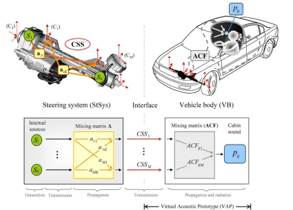
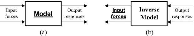
Figure 1.1: The physical problem behind steering induced noise in vehicles

The physical domain can be modelled as a multiple input single output (MISO) system: Several different source mechanism, sk (k=1...K), act as inputs of the system and, according

to the mixing and filtering matrices A and ACF accounting for related transmission, propagation and radiation processes within the steering system and the vehicle body respectively, contribute in varying degree to the single sound at the driver’s ear, pR. Note, the

system model in Figure 1.1 is depicted in most general form to allow approaching the problem in time domain as well as in frequency domain. In time domain the matrices A and ACF perform convolutive mixing to their respective input signals whereas linear mixing is assumed in frequency domain.

From an engineering point of view it makes sense to separate the physical domain into two sub-domains, the steering system (StSys) and the vehicle body including the air space inside the cabin (VB). Both parts are coupled through several physical links. Physical links in this respect only account for mechanical but not for acoustical or vibro-acoustical coupling. In reality, such links are usually formed by rigid connections between the steering system and the remaining vehicle structure, e.g. bolting of StSys and sub frame (Figure 1.1-(C1)),

connections between StSys and tie rods (C2) or coupling of StSys and steering column (CM)

vibrational energy can be transmitted from the steering system into the vehicle body. At the same time, this interface separates the part of the physical domain that is in the range of control for designers and engineers at ZFLS (StSys) from the non-controllable part (VB). Although the design targets for engineers at ZFLS are defined only for the steering system, both parts have to be considered in order to achieve auralisation of the interior sound which is required to judge NVH quality.

In Bauer’s aforementioned VAP [7], the steering system is assumed as ‘black box’ which is characterised by its ‘external properties’ at the interface to the vehicle. Doing so, no detailed information about the structure-borne sound processes inside this box is necessary. A VAP is achieved by relating the external dynamic properties of the steering system (CSS) and the properties of the conducting vehicle body (ACF) to the cabin sound (p), using equation (1.1). It has been shown [7] that the external properties of a steering system can be characterised independently of a receiver structure, allowing to measure its source strength in arbitrary physical assemblies, e.g. when connected to a test bench. For this purpose, the component source strengths (CSS) has to be expressed in terms of blocked forces obtained in-situ by employing frequency domain inverse techniques [17],[18]. Transmission, propagation and radiation processes taking place inside the conducting vehicle body are accounted for by using vibro-acoustic transfer functions (ACF), measured in a real vehicle between the connection points of the StSys and a point inside the compartment coinciding with the head position of the driver. Although auralisation can be achieved in this way, the usability of this VAP for noise control engineers with respect to minimizing ‘perception of a fault’ (PF) by design is limited. The major shortcoming of this approach is, that neither the internal source mechanisms (sk) nor the internal mixing and filtering processes (A) inside the steering system

are considered.

Gaining this information is the aim of the presented research project. Concerning the source mechanisms (sk), the internal transient sound sources within electrical steering systems are to

blocked forces at the interface to the vehicle. The external quantities (CSS) composed of sk

and A then could be auralised using Bauer’s VAP [7].

Providing such a detailed VAP, noise control engineers were able to rank order the internal transient sound sources according to their partial contribution to the perceived interior vehicle sound. In this way, dominating internal sources could be identified and optimised first, before focussing on weak contributing sources that may influence PF only moderate. Applying a detailed VAP of a steering system would further provide essential insight into the internal generation, transmission and propagation processes of transient structure-borne sound in electrical steering systems. This comprehension could help engineers to evaluate whether primary modifications on the active sources or secondary actions on the conducting passive structure are necessary for minimizing PF. Clearly, such a sophisticated VAP, allowing users to figuratively ‘look into the steering system’ instead of studying the overall vibro-acoustic behaviour of the entire assembly, would be innovative and could offer many other advantages for various noise control tasks, too.

1.5.

Time domain representation of electrical steering systems

Having disclosed the physical problem of steering induced transient sound in vehicles, the question of how best to address it remains. As elaborated, sources and transfer paths are to be characterised independently of each other and auralisation based on the combination of these characteristics should be possible. Each of these issues is challenging and various solutions of different level of sophistication to each matter can be found in literature. Most of them employ techniques in which the physical problem is represented either in frequency domain or time domain. Favouring one representation over the other depends on the specific application and the particular motivation.

It is believed that the problem of transient sound in vehicles originated within electrical steering systems can be best approached in time domain. The motivation for this hypothesis is explained in the following.

mechanical phenomena, such as colliding assemblies for instance. Hence, structural and acoustic responses provoked by the internal forces also carry transient features, so that tackling the problem in time domain is favoured.

Second, the source characterisation issue poses an inverse problem since neither the transient excitation forces inside the steering system (sk) nor the external dynamic (blocked) forces

acting at the interface to the vehicle connections (CSS) can be measured directly. Commonly, such ill-posed inverse problems are addressed in frequency domain where matrices containing measured frequency response functions (FRFs) have to be inverted. Yet, these methods are well known to suffer from poor conditioning and to be highly sensitive to measurement noise. Although the robustness of the solutions may be improved with some form of regularisation (see amongst many examples [20],[21]), usually significant effort and expertise is to be directed to obtaining satisfying results. Regarding possible applications of VAPs for NVH engineers, this special know-how cannot be expected.

Third, the transfer paths between the internal transient sound sources and the external connection points of the steering system are to be characterised. Although the structural dynamic properties at the external interface to the vehicle have proved to be invariant on the steering angle [7],[8], it is not known if the internal transfer path may vary in time due to dynamic steering. If so, employing time domain modelling techniques could be advantageous to account for the time-varying nature of the internal dynamic properties. It is noted that dynamic steering will not be considered within this research project.

literature, e.g. by artificially increasing the number of data points of the synthesised spectrum by spectral interpolation [6] or adopting computationally intensive hybrid approaches in which frequency domain methods are used to gain transfer functions of the passive components (ACF) that first are transformed into time domain FIR filters before synthesis and auralisation is carried out by convolution with recorded source strength time histories (CSS) ([7], [8]). However, it is argued that a VAP directly represented as time domain model in this context would be more straightforward. First, it is believed that auralisation carried out solely with time domain data could avoid most of the above mentioned problems. Audible sounds of any length could simply be generated by directly convolving the temporal data of the passive structure (ACF) with the time data of the active sources, the latter representing time dependent CSSs captured for an arbitrary operating time. In this way, general problems due to converting data from frequency domain into time domain could be avoided completely. Second, time domain VAP models would possibly better allow for relating time dependent passive data (ACF), e.g. steering angle dependent transfer functions, to specific causative events in the captured source data (CSS).

Finally, since perception is generally dependent on the time signature of a noticed sound [1], capturing a signal’s temporal waveform throughout all evolutionary stages, i.e. generation, transmission, propagation and radiation, may provide additional important information to noise control engineers.

1.6.

Thesis objectives

To provide useful guidance for addressing the problem of transient structure-borne sound originated within electrical steering systems and the associated problem of perception of a fault, the following aims have to be achieved:

• Identification of internal transient sound sources:

• Development of a measurement strategy:

In order to provoke internal transient generating forces, external excitations need to be applied to the steering system. Therefore, a strategy has to be evaluated that allows applying controlled external excitation forces to the steering system. The concept needs to consider that all measurements have to be carried out while the steering system is coupled to another structure, e.g. a test bench, which is required to provide this external excitation. Thus, in-situ measurement techniques have to be used.

• Independent characterisation of the internal sources:

To independently characterise the transient sound sources within real steering systems a concept and a practicable approach have to be developed that allow the individual strength of each structure-borne sound source to be quantified, ideally in terms of time domain blocked forces obtained from measurements carried out in-situ. This task poses several challenges. First, a general time domain routine being able to provide robust and accurate solutions to the associated inverse problem has to be established. The method should allow for simultaneously reconstructing multi-channel (blocked) force time signatures based on measured data so that it is applicable even for sophisticated technical structures, such as steering systems. Second, since the time domain routine is used to quantify the individual strengths of each internal transient sound source from measured data, numerical tools shall be achieved that can be employed to evaluate the quality of this measured data. In this way, defective data can be detected before carrying out the inversion algorithm. Theoretical and practicable feasibility are to be tested in both cases.

• Relating internal transient sources to external properties:

The contributions from all independent internal sources have to be related to external properties (blocked forces) determinable at the connection points of the steering system. As can be seen from Figure 1.1, this relationship is given by the mixing and filtering matrix A. A philosophy and a practicable approach are to be developed allowing for quantifying the mixing coefficients of this matrix. If both, the internal sources (sk) and the mixing matrix (A) are identified, a model of the physical system

be employed in order to investigate the influence of each internal transient sound source on the perceived sound inside the vehicle cabin.

• Validation of the obtained methodology based on test bench measurements.

Chapter 2

Literature review and theory

2.1.

Introduction

In the previous chapter the problem of transient structure-borne sound and the associated phenomenon of perception of a fault (PF) within electrical steering systems were discussed. In this respect, independent characterisation of the transient sound sources inside the steering system was stressed to be one of the most fundamental tasks to be achieved within this study. Being able to quantify the activity of the internal sources as well as the respective transmission paths between each source and the connection points at which the steering system is coupled to a supporting structure, e.g. a vehicle body or a test bench, would provide important information to designers and engineers and may serve as initial guidance in order to reduce PF by design.

transmission theoretically requires consideration of all kinds of coupling between the different contact points, i.e. transfer, cross and cross-transfer mobilities are to be considered [24].

Moreover, to fully quantify structure-borne sound transmission from the source into the receiver in theory all of the causative forces and moments have to be considered. However, on account of several practical limitations direct measuring the interfacial forces and particularly the moments is rarely possible. Instead, inverse methods may be employed that allow inferring the causative quantities from more accessible quantities, like structural responses, which are representative for the effects of the physical problem [28]. Since the source characterisation problem in this way may emerge as an ill-posed inverse problem, severe numerical difficulties have to be dealt with in order to obtain robust solutions [28],[29] required to achieve reliable quantification of the respective source activities. Additional challenges inherent in the source characterisation problem result from the need to quantify active sources independently of a connected receiver structure. In the context of transient structure-borne sound, as in the case of electrical steering systems, the ambition to achieve a description of the source activity in time domain (see section 1.5) further increases the complexity of the general source characterisation problem.

Since all of the presented techniques invoke concepts relying on linear and time invariant (LTI) system theory a brief discussion on the assumption of LTI behaviour for electrical steering systems subjected to internal transient sound generation is provided in the following.

2.2.

Assumption of linear and time-invariant system behaviour

All methods presented and used in this study invoke principles and concepts based upon linear and time invariant (LTI) system theory. In the context of steering induced transient structure-borne sound assuming LTI behaviour may however be controversial. The generation of transient structure-borne sound is caused by some form of mechanical excitation inside the steering system (StSys) which sometimes may be construed as being related to time varying or even nonlinear system behaviour. Considering the phenomenon of rattling for example, transient forces are provoked inside the steering gear by impacting assemblies due to load-dependent short-time lifting and abrupt equalising movements between adjacent components (see section 3.3.3). The associated non-deterministic processes of interfacial movement, occurrence of clearance as well as possible transitory changes in the local physical properties of the structure (i.e. dynamic mass, stiffness and damping) point towards nonlinear, rather than linear, system behaviour [30]. If furthermore dynamic steering is considered, the transmission paths between the internal source regions and any point on the coupled source-receiver system, e.g. StSys connected to a test bench or a vehicle body, may vary with time so that again the strict LTI assumption is violated.

On the other hand, considering the StSys explicitly as a nonlinear and time-varying dynamic system is believed to be over-constrained and, moreover, would exceedingly exacerbate tackling the problem of steering induced transient sound. This is due to the fact that no unique analytical or experimental approach to deal with nonlinear system identification is available [30],[31],[32] and modelling of time-varying system properties for sophisticated technical structures is generally difficult, in particular when non-deterministic and fast varying mechanisms are to be dealt with.