International Journal of Emerging Technology and Advanced Engineering
Website: www.ijetae.com (ISSN 2250-2459, Volume 2, Issue 10, October 2012)378
Estimation of Governing Parameters of the Structure
Subjected To Ground Motion Using Transfer Function
Approach
Sathe Prashant Dasharath
1, Ashok Kumar
2and S.K.Thakkar
3 1Assistant Professor, MAEER’S MIT Pune,2Professor, Indian Institute of Technology Roorkee, 3Retired Professor, Indian Institute of Technology Roorkee, 1[email protected],2[email protected]
Abstract—The present paper describes, estimation of the
governing parameters for linear structural system subjected to ground motion using transfer function approach through frequency domain analysis. The transfer functions were determined by finding Fourier Transform of its responses for synchronous noise input. Synchronous noise is a broad band time series, which looks like random noise but has an absolutely flat power spectrum. The response for the linear structural system using frequency domain analysis through the transfer function approach for earthquake excitation discussed here showed that the same level of accuracy as that of linear modal time history analysis using commercial software. So once we have found the transfer function of the structure responses then if there is earthquake of recorded accelerogram in future then by multiplying the transfer function with the Fourier Transform of earthquake time history we can obtain the response of that particular element. Thus, if we can archive different transfer functions of the structure then we will not require the detailed modeling of the structure for future earthquake.
Keywords—Frequency domain, Transfer function,
Synchronous noise, Dynamic Analysis, Inter-Storey Drift
I. INTRODUCTION
To carry out the design of structures subjected to dynamic loads the engineer have available either time domain or frequency domain methodologies; which approach is going to be used is case-dependent [1,2].
Time domain approaches [1-6] are very much used in daily structural engineering practice as they can provide the required response in most cases and are very much familiar to structural engineers. In addition, nowadays there is a great deal of commercial codes available, based on time domain approaches, which include a great variety of strategies for linear and non-linear analyses, and have excellent pre- and post-processing modules which simplifies enormously the daily design activities. The same time domain algorithms are applied now days to carry out dynamic analyses in areas close to structural engineering.
Frequency domain approaches, which are based on Fourier transform ([1, 7–8] etc.), are equivalent to time domain procedures in a great deal of applications and more adequate in many others. One case when frequency domain procedures must be preferred is that in which physical properties are better described in the frequency domain. Structural damping parameters, which can be easily established in the frequency domain, are traditionally represented in time-domain approaches via equivalent viscous damping constants; these two models are equivalent only at the natural frequency [1]. Another situation in which frequency domain approaches are frequently used concerns soil–structure interaction problems; a great deal of technical papers on this topic (see [9], for instance) have published tables and simple algorithms from which engineers can obtain frequency dependent soil parameters.
International Journal of Emerging Technology and Advanced Engineering
Website: www.ijetae.com (ISSN 2250-2459, Volume 2, Issue 10, October 2012)379
II. FREQUENCY DOMAIN METHOD
In this work, transfer function in frequency domain is
obtained analytically for MDF system, which is then
convoluted with Fourier transform of excitation to get
the Fourier transform of the response, which on
inverse Fourier transform yields response in time
domain.
A. Analytical Transfer Functions
For linear SDOF systems and following are steps of this method.
1. First find the Fourier transform F(ω) of the input excitation function f(t) and then find the transfer function of the system H(ω) . For SDOF system, transfer function can be found out using equation of motion in frequency domain.
2. Product of these two functions at each frequency interval in frequency domain will yield Fourier transform of response.
V(ω) = F(ω) . H(ω) (1) 3. Then Inverse Fourier transforms of the product, is
the response of the system, v(t). Mathematically,
( ) ∫ ( ) (2)
( ) ∫ ( ) (3)
which, is equivalent to complex frequency response function of SDOF system,
( ) ( ) (4)
The response of the system i.e. inverse transfer function
V(ω) is
( ) ∫ ( ) ( ) (5)
B. Discrete Fourier Transform
Evaluation of the Fourier transform is tedious as it involves complex integral; hence, numerical evaluation of the transforms is particularly possible.In addition, the Fourier transforms of the unit impulse response function are only available in discrete form at regular interval of time.
Therefore, develops a Fourier, discrete Fourier transform to relate continuous and discrete transforms.
Let, excitation function f(t) is time function at N equal interval.
n= 0, 1, 2, 3, N-1 and time interval, t=0, Δt, 2Δt… (N-1) Δt. With time period, T=N. Δt and frequency, Δ = 2 /T Now, periodic extension of function at T = N. Δt
( ) ∑
( ) (6)
Hence, discrete Fourier transform of the f(t) is,
( ) ∑
( ) (7)
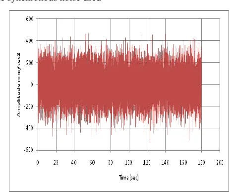
C. Synchronous Noise
A broadband time series, which looks like random noise but has an absolutely flat power spectrum, is known as synchronous noise [10, 11]. To generate synchronous noise, a constant is loaded into an array corresponding to nonzero spectral bins of an inverse discrete Fourier transform (IDFT). The IDFT of this data set will be a sequence which will be Drichlet kernel having high crest factor (ratio of peak to rms value). To reduce the crest factor, phase of the spectral terms is uniformly randomized. This requires use of random number generator to get numbers between -1 and 1. A random number is picked which is taken as a real part of the IDFT array and its corresponding imaginary part is calculated such that a magnitude is a constant number (say 1). Similarly, other pairs of real and imaginary parts of IDFT arrays are constructed such that magnitude of each pair is constant. Thus, the array comprises of constant magnitude and random phase of each pair. IDFT of this data set yields synchronous noise that has an approximate Gaussian density function and a crest factor of about 3.
However, in this work random phase and FFT algorithm for IDFT has been used to get the synchronous noise. Step by step method to generate synchronous noise of 18,000 samples is as follows and a typical synchronous noise is shown in Fig.1.
1. Pick a random number between –1 and 1 as real part of IFFT array.
International Journal of Emerging Technology and Advanced Engineering
Website: www.ijetae.com (ISSN 2250-2459, Volume 2, Issue 10, October 2012)380
3. Pick another random number and generate 9001 such pairs corresponding to first 9001 bin frequencies (Nyquist frequency).
4. For bin numbers 9002 to 18000, real part are found by taking mirror image of real part of the set upto Nyquist frequency.
5. For bin numbers 9002 to 18000, imaginary parts are found by taking negative of mirror image of imaginary parts of the set upto Nyquist frequency.
6. Inverse FFT is then performed on these 18000 pairs of real and imaginary parts, which yield the desired synchronous noise.
[image:3.612.59.292.291.484.2]The synchronous noise used
Figure 1: Synchronous Noise
D. Transfer Function Using Synchronous Noise Input
Transfer function in frequency domain of any system is defined as Fourier transformation of response divided by Fourier transformation of excitation. Let F(ω) be the Fourier transform of excitation f(t) at an t discrete frequency and let
F(ω) = a + ib (8) where a is the real part of F(ω) and b is the imaginary part of F(ω).
Let V(ω) be the Fourier transform of response of system
v(t) at any discrete frequency ω and
V(ω) = c + id (9) where c is the real part and d is the imaginary part of V(ω).
Then, transfer function of the system H(ω) at any discrete frequency ω is given by
( ) ( ) ( ) (10)
( ) ( )( ) (11)
( ) (12)
Hence, the amplitude of the above equation can be given as
2 2 2
2
2 2
ˆ
b a
c b d a b a
d b c a
H (13)
Theoretically, giving any random excitation to the system and finding its response can be used to find out transfer function of any system. However, problem with using any random excitation is that the denominator of Eq.(13) for some discrete frequencies may become nearly zero causing problem of division by zero. Here, the use of synchronous noise as input excitation becomes very handy because in synchronous noise the term a2+b2 will always be unity at all discrete frequencies and thus an accurate transfer function can be found out at all the frequencies.
III. NUMERICALEXAMPLE
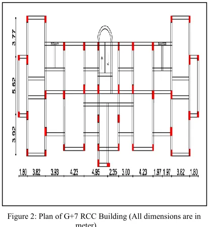
A. Description of the Building
The Building under consideration is G+7 storied Reinforced Cement Concrete building. It is located in Roorkee, which comes under seismic zone IV.Total height of the building is 25.630 m above ground level with storey height 3.580 m for ground storey and 3.150 m for remaining storey. Plan dimension of the building is 14.350
International Journal of Emerging Technology and Advanced Engineering
Website: www.ijetae.com (ISSN 2250-2459, Volume 2, Issue 10, October 2012)381
Superstructure of the building has been analyzed by using 3D space frame model in SAP2000 V11. Stiffness of the brick infill is not taken into the account but its weight is being considered i.e. bare frame analysis is made. Staircase is centrally located but is separated from the main structure, so its stiffness is not taken into account. Grade of the concrete used for the construction is M25 and the grade of the steel is Fy415.
[image:4.612.83.289.246.471.2]Fig. 2 shows the plan of the considered RCC building (G+7) is
Figure 2: Plan of G+7 RCC Building (All dimensions are in meter)
Material densities have been taken as per IS: 875 (Part I) and are presented below.
Density of the Concrete = 25 kN/m3 Density of the Masonry = 20 kN/m3
For the building we have selected the total dead load is being 63,486.970 kN.
Live load on the building is taken as per provisions given in IS: 875 (Part II).
Following load combinations are considered for the modal time history analysis of the building as per IS1893 (Part-1)-2002.
TABLE I
LOAD COMBINATIONS
Sr. No. Load Combination
1 1.5(DL+LL)
2 1.2(DL+LL EQ)
3 1.5(DL EQ)
4 0.9DL 1.5EQ
Assumptions made in Dynamic Analysis are as follows:
1. The bases of the frames are assumed as fixed with respect to rotational and translation movements. 2. Neglecting effect of stiffness of infill, bare frames
are analyzed.
3. Damping of the structure is assumed to be constant as 5% of the critical.
4. Members of the structures are assumed to be homogeneous, isotropic.
5. Elastic modulus in tension and compression is assumed to be same.
For the dynamic analysis of the building, the gravity load that is applied on the structure is shown below in Table 2.
TABLE II
GRAVITY LOAD ON THE BUILDING
Sr.No. Load Description Reaction (kN)
1 DEAD 18172.860
2 DEAD-WALL 30127.590
3 DEAD-SLAB 11804.460
4 DEAD-FF 2786.710
5 DEAD-RT 595.350
6 LIVE 8334.320
International Journal of Emerging Technology and Advanced Engineering
Website: www.ijetae.com (ISSN 2250-2459, Volume 2, Issue 10, October 2012)382
B. Free Vibration Analysis Results
The free vibration analysis of G+7 RCC building has made using SAP2000 V11 software. The time periods and frequencies of the building for first 12 modes are shown in Table 3. The fundamental time period is 1.265 second. The time period varies from 1.265 second to 0.119 second for twelfth mode.
TABLE III
TIME PERIOD AND FREQUENCY OF (G+7) RCC BUILDING
Mode Period (Sec) Frequency (Cycle/sec)
1 1.265 0.790
2 0.892 1.121
3 0.845 1.184
4 0.407 2.459
5 0.295 3.385
6 0.280 3.570
7 0.224 4.457
8 0.164 6.089
9 0.157 6.373
10 0.152 6.583
11 0.120 8.366
12 0.119 8.408
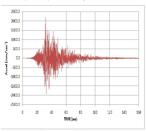
[image:5.612.324.577.114.343.2]The linear modal time history of the G+7 RCC building is made using SAP2000 V11 software. Response such as displacement, bending moment of the building was determined for excitation input of synchronous noise of 180 second duration and sampling rate of 100 using SAP2000 V11 software. Transfer function in frequency domain of the building response was then determined using Eq. (12).This transfer function was then convoluted in frequency domain with Fourier Transformation of the accelerogram of Fig.3 and then inverse Fourier transformation done to get the time domain response of structure. The HKD-EW is the time history of earthquake which was generated in Shintoku, Tokachi District, Japan in 26 September 2003, 04:50am having PGA= 0.23 g m/sec2 The HKD-EW time history (mm/sec2) is used for comparison of response through time history analysis using SAP2000 V11 and frequency domain using transfer function approach shown below in Fig.3.
Figure 3: HKD-EW Time History
IV. RESULT AND DISCUSSION:INTER STOREY DRIFT FOR
1ST-2NDF LOOR
The inter storey drift for 1st -2nd floor joints i.e. J24-J26 is calculated using linear modal time history analysis and transfer function approach in frequency domain. The graphs of transfer function that are symmetrical about 50
Hz and comparisons between the results of response from the transfer function approach and direct through linear modal time history are given below.
Drift for 1st and 2nd floor:
Figure 4(a): Transfer function EXUXJ24&26
0 0.01 0.02 0.03 0.04 0.05 0.06 0.07 0.08 0.09
0 5 10 15
Gai
n
[image:5.612.327.558.494.692.2]International Journal of Emerging Technology and Advanced Engineering
Website: www.ijetae.com (ISSN 2250-2459, Volume 2, Issue 10, October 2012)383
Figure4 (b): Comparison between the result from the transfer function and SAP software
TABLE IV
PERCENTAGE ERROR IN BETWEEN TRANSFER FUNCTION APPROACH IN FREQUENCY DOMAIN AND SAP2000V11 IN TIME DOMAIN ANALYSIS RESULTS OF INTER
STORY DRIFT
Description Time(sec) Transfer Function SAP
% Error (with respect to
transfer function approach
DRIFT 1st-2nd Floor(mm)
32.840 19.050 19.390 -1.800
33.430 -17.630 -18.160 -3.010
The inter storey drift for 1st -2nd floor joints i.e. J24-J26 is calculated using linear modal time history analysis and transfer function approach in the frequency domain. The maximum percentage of error with respect to transfer
function approach is -3.010% from Table 4. The responses found through above transfer function approach in frequency domain matches well with that found directly using commercial software SAP2000 V11. The inter storey drift for 1st – 2nd floors has maximum peak of gain at frequency 0.789 Hz and the maximum value of it is 19.050
mm which exceed 0.004 times the storey height i.e.12.600
mm. Thus it is not safe as per IS 1893-2002.
V. CONCLUSION
In this work, transfer function of response like inter storey displacement of G+7 RCC building were found out using synchronous noise input. Transfer function so determined was then used to find response of building for HKD-EW time history. It has been shown here that the response found through above transfer function approach in the frequency domain matches well with that found directly using commercial software SAP2000 V11.
Once we have found the transfer function of the building responses like for bending moment, shear force, displacement, inter storey drift then if there is earthquake of recorded accelerogram in future then by multiplying the transfer function with Fourier Transform of earthquake time history we can obtain responses of that particular element. Thus, if we can archive different transfer functions of the building then we will not require the detailed modeling of the building for future earthquake. For the damage detection and system identification this frequency domain approach can be used.
REFERENCES
[1] Bathe K.J.(1996). Finite Element Procedures, Prentice-Hall, Englewood Cliffs, New Jersey.
[2] Clough R.W., Penzien J.(1993).Dynamics of Structures, second ed., McGraw-Hill, New York.
[3] Harris F.J.(1987). Time Domain Signal Processing with the DFT, Handbook of Digital Signal Processing Engineering Applications, Edited by Douglas F. Elliot, Academic Press, Tavel, P. 2007 Modeling and Simulation Design. AK Peters Ltd.
[4] Hughes T.J.R.(1987). The Finite Element Method, Dover Publications Inc., New York.
[5] Kumar A., Basu S., Chandra B.(2000). Use of Synchronous Noise as Test Signal for Evaluation of Strong Motion Data Processing Schemes, Proceedings 12th World Conference on Earthquake Engineering, Auckland, New Zealand, 0931.
[6] Paz M.(1997). Structural Dynamics––Theory and Computation, fourth ed., Chapman and Hall, New York.
[7] Veletsos A., Ventura C.(1984). Efficient Analysis of Dynamic Response of Linear Systems, Earthquake Engrg. Struct. Dynam.,12 (521–536).
-25.0 -20.0 -15.0 -10.0 -05.0 00.0 05.0 10.0 15.0 20.0 25.0
0 50 100 150 200
D
ri
ft
EX
UXJ
26&
24,
1S
T
&
2ND
FLO
OR
(m
m
)
Time (sec)
DRIFT TRANS HKD -EW
International Journal of Emerging Technology and Advanced Engineering
Website: www.ijetae.com (ISSN 2250-2459, Volume 2, Issue 10, October 2012)384
[8] Veletsos A., Ventura C.(1985). Dynamic Analysis of Structures by the DFT Method, J. Struct. Engrg. ASCE 111 (2625–2642). [9] Weaver W.Jr., Johnston P.R.(1987). Structural Dynamics by Finite
Elements, Prentice-Hall, Englewood Cliffs, New Jersey.
[10] Wolf J.P.(1985). Dynamic Soil–Structure Interaction, Prentice-Hall, Englewood Cliffs, New Jersey.