Improved membrane absorbers

(1)

IMPROVED MEMBRANE

ABSORBERS

Robert Oldfield

Research Institute for the Built and Human Environment, Acoustics

Department, University of Salford, Salford, UK

(2)

ACKNOWLEDGEMENTS

I would like to express my thanks to Prof. Trevor Cox for his inspirational supervision, guidance and time during this project. Also I would like to thank everyone in the Acoustics department at the University of Salford for their continual support, encouragement and suggestions with particular thanks to Fouad and the team of G61. Thanks also to Dr. Mark Avis for his practical suggestions and willingness to offer help whenever it was needed.

(6)

ABSTRACT

This thesis presents research into two novel techniques for improving the low frequency performance, tunability and efficiency of membrane absorbers. The first approach uses a loudspeaker surround as the mounting for the membrane, increasing the moving mass, thereby lowering the resonant frequency of the system. Using a loudspeaker surround also allows for more accurate prediction of the absorber’s performance as the mounting conditions are such that the membrane can be more accurately represented by a lumped mass moving as a piston.

(7)

GLOSSARY OF SYMBOLS

B Magnetic flux density (T)

Bl Force factor (Tm)

A

C Acoustic compliance (m5N-1)

AB

C Acoustic compliance of the cabinet (m5N-1)

AD

C Compliance in acoustic units of the diaphragm (m5N-1)

AEV

C Capacitance in acoustical units as a result of variable inductor LEV

AT

C Total acoustic compliance (m5N-1)

1

AE

C Capacitance in acoustical units as a result of inductor L1

2

AE

C Capacitance in acoustical units as a result of inductor L2

E

C Electrical capacitance (F)

EV

C Variable electrical capacitance (F)

M

C Mechanical compliance

MD

C Mechanical compliance of the diaphragm without an air load (mN-1₎

MS

C Mechanical compliance of the diaphragm with an air load (mN-1)

F Force (N)

f Frequency (Hz)

i Electrical current (Ω)

j −1

k Wavenumber (m-1)

M

k Mechanical stiffness (Nm-1₎

l Length of coil (m)

E

L Electrical inductance (H)

AEV

L Inductance in acoustical units as a result of capacitor CEV

M Mass (kg)

AB

M Acoustic mass at the back of the diaphragm (kgm4)

AD

M Acoustic mass of the diaphragm without an air load (kgm4)

AF

M Acoustic mass at the front of the diaphragm (kgm4)

AS

(8)

AT

M Total acoustic mass (kgm4)

MD

M Mechanical mass of diaphragm without air load (kg)

MS

M Mechanical mass of diaphragm with air load (kg)

in

p Input acoustic pressure (Pa)

q Electrical charge (C)

AB

R Acoustic resistance/damping at the back of the diaphragm (Nsm-5)

AD

R Acoustic resistance/damping of the diaphragm without an air load (Nsm-5)

AE

R Resistance in acoustical units as a result of resistor RE

AEV

R Resistance in acoustical units as a result of resistor REV

2

AE

R Resistance in acoustical units as a result of resistor R2

AF

R Acoustic resistance/damping in front of the diaphragm (Nsm-5)

AS

R Acoustic resistance/damping of the diaphragm with an air load (Nsm-5₎ AT

R Total acoustic resistance/damping (Nsm-5)

E

R Electrical resistance of loudspeaker coil (Ω)

EV

R Variable electrical resistance (Ω)

M

R Mechanical resistance/damping (Nsm-1)

MD

R Mechanical resistance/damping of diaphragm without air load (Nsm-1)

MS

R Mechanical resistance/damping of diaphragm with air load (Nsm-1)

S Area (m2)

D

S Area of diaphragm (m2)

t Time (s)

U Volume velocity (m3s-1)

u Particle velocity (ms-1)

V Volume (m3)

v Voltage (V)

in

v Input voltage (V)

B

V Volume of cabinet (m3)

x Displacement (m)

A

Z Acoustic impedance (Pasm-1 or MKS rayl)

AB

(9)

F

A

Z Acoustic impedance at the front of the diaphragm (Pasm-1 or MKS rayl)

E

Z Electrical impedance (Ω)

M

Z Mechanical impedance (Nsm-1)

α Absorption coefficient

λ Wavelength (m)

ρ Density (kgm-3)

0

ρ Density of air (1.21kgm-3) ω Angular frequency (s-1)

(10)

LIST OF TABLES

Table 5.1 Summary of the impedance analogue ...75

Table 5.2 Summary of the mobility analogue...76

LIST OF FIGURES Figure 2.1 Reflection of a sound wave incident normal to a surface ...7

Figure 2.2 a) Closed cell foam, no propagation path through absorbent as pores are closed and unconnected. b) Open celled foam, interconnected pores allow for acoustic propagation and consequent thermal/viscous losses. (From Cox and D’Antonio [8]) ...10

Figure 2.3 Test apparatus for measurement of flow resistivity ...13

Figure 2.4 Diagram of sound propagation through multiple layers...16

Figure 2.5 Schematic representation of a typical Helmholtz absorber...20

Figure 2.6 Diagram of a Helmholtz type acoustic resonator...20

Figure 2.7 Schematic representation of a standard membrane absorber ...22

Figure 2.8 Diagrammatic representation of the transfer matrix modeling of sound incident to a membrane absorber ...26

Figure 2.9 Transfer matrix modeling of porous absorbent with a rigid backing using the Delany and Bazley model ...27

Figure 2.10 Transfer matrix prediction of a simple membrane absorber ...28

Figure 3.1 Diagram of the typical setup of an impedance tube using the standing wave method...33

Figure 3.2 Diagram of the typical setup of an impedance tube using the transfer function method ...36

Figure 3.3 a) Photograph of completed impedance tube b) Schematic of completed impedance tube ...41

Figure 3.4 Impedance tube for the transfer function method with modeled image source technique ...43

Figure 3.5 Image source technique for multiple microphone positions ...44

Figure 3.6: Plot showing the validity of the generalised version of Cho’s least-square optimisation method. Note that the measured plot was obtained by manually overlapping the measured data for each microphone pair according to the corresponding frequency range each best describes. ...46

Figure 3.7: Results for absorption coefficient of a 12cm thick sample of mineral wool as measured in the large low frequency impedance tube and a smaller high frequency tube...47

Figure 4.1 Schematic representation of a simply supported plate...50

Figure 4.2 Schematic representation of a clamped plate ...51

Figure 4.3 Schematic representation of a freely supported plate...51

Figure 4.4 Schematic presentation of pistonic mounting ...52

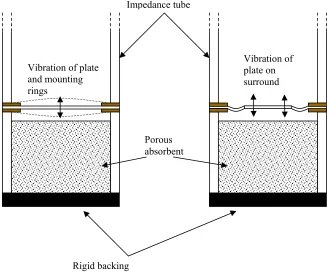
Figure 4.5 Photos of membrane mounting ...54

Figure 4.6 Experimental setup for the accelerometer tests...55

Figure 4.7 Results from the accelerometer tests...56

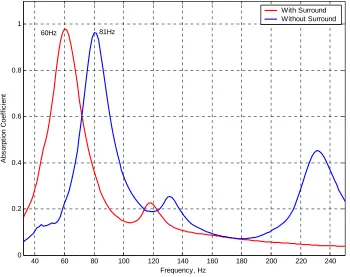
Figure 4.8 Results from impedance tube tests with and without surround in large sample holder ...57

(11)

Figure 4.10 Samples mounted in impedance tube, demonstrating how mounting rings

can support modal behaviour ...59

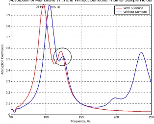
Figure 4.11 Results from impedance tube tests with and without surround in small sample holder ...60

Figure 4.12 Results from impedance tube tests on hardboard with and without surround in small and large sample holders ...61

Figure 4.13 Equivalent circuit for a membrane absorber ...62

Figure 4.14 Experimental setup for measuring compliance of surround...63

Figure 4.15 Results from experiment to determine compliance of surround ...64

Figure 4.16 Absorption curve from equivalent circuit model of membrane with and without surround ...66

Figure 4.17 Comparison of measured absorption curves with predictions from a transfer matrix model ...67

Figure 5.1 Simple representation of the electrical section of a loudspeaker ...77

Figure 5.2 More complicated representation of the electrical section of a loudspeaker 78 Figure 5.3 Mechanical representation of a loudspeaker ...80

Figure 5.4 Impedance analogue circuit of the mechanical section of a loudspeaker ...81

Figure 5.5 Mobility analogue circuit of the mechanical section of a loudspeaker...81

Figure 5.6 Impedance analogue circuit of the acoustical section of a loudspeaker...82

Figure 5.7 Mobility analogue circuit of the acoustical section of loudspeaker used as a membrane absorber ...83

Figure 5.8 Idealised transformer...84

Figure 5.9 Simplified idealised transformer ...84

Figure 5.10 Equivalent circuit linking electrical, mechanical and acoustical sections with transformers ...86

Figure 5.11 Equivalent circuit of membrane absorber with electrical and mechanical sections combined ...86

Figure 5.12 Equivalent circuit of membrane absorber with electrical, mechanical and acoustical sections combined ...87

Figure 5.13 Equivalent circuit of membrane absorber in impedance analogue ...87

Figure 5.14 Simplified equivalent circuit of membrane absorber ...90

Figure 5.15 Comparison of equivalent circuit model with impedance tube measurements...92

Figure 5.16 Real part of surface impedance from both predicted and measured data....93

Figure 5.17 First three vibrational modes of a circular plate...94

Figure 5.18 Multi-plot of absorption and surface impedance showing the first two resonant modes of the loudspeaker ...95

Figure 6.1 Electrical section of the absorber equivalent circuit with an additional variable resistor across terminals A and B....101

Figure 6.2 Full equivalent circuit of absorber with additional variable resistor across terminals...101

Figure 6.3 Simplified equivalent circuit of absorber...101

Figure 6.4 Changes in absorption curves with a variable resistor connected across loudspeaker terminals...103

Figure 6.5 Mounting of loudspeaker in large sample holder for impedance tube testing ...104

Figure 6.6 Measurements made on absorber in impedance tube changing resistive load on loudspeaker terminals ...105

(12)

Figure 6.8 Predicted absorption coefficient changing the resistive load on the absorber without porous absorption in cabinet. ...107

Figure 6.9 Measured absorption coefficient of absorber with variable resistive load with porous absorption in the cabinet ...108

Figure 6.10 Equivalent circuit with additional variable capacitor connected to

loudspeaker terminals...110

Figure 6.11 Predicted absorption curves with a variable capacitor connected to

loudspeaker terminals...111

Figure 6.12 Measured absorption curves, changing the load capacitance connected across loudspeaker terminals...111

Figure 6.13 Equivalent circuit modelling a variable resistor in series with a variable capacitor connected to the terminals of the loudspeaker ...114

Figure 6.14 Multi-plot showing changes in the trend of absorption for different

combinations of resistors in series with capacitors...115 Figure 6.15 Equivalent circuit modelling a variable capacitor in parallel with a variable

resistor connected to the terminals of the loudspeaker ...116

Figure 6.16 Equivalent circuit modelling a variable inductor connected to the terminals of the loudspeaker ...117

Figure 6.17 Absorption curves changing inductive load on loudspeaker...118

Figure 6.18 Equivalent circuit modelling a variable inductor in series with a variable capacitor connected to the terminals of the loudspeaker ...119

Figure 6.19 Multi-plot of absorption trends with a variable inductive and capacitive load connected in series ...120

Figure 6.20 Equivalent circuit modelling a variable capacitor in parallel with a variable inductor connected to the terminals of the loudspeaker...121

Figure 6.21 Multi-plot showing predicted absorption trends with a variable inductor and capacitor connected in parallel to the terminals of the loudspeaker ...122

Figure 6.22 Equivalent circuit of absorber system with simplified motor impedance terms and variable capacitor connected to terminals ...125

Figure 6.23 Resonant frequency versus capacitance value to determine the component value needed for a given resonant frequency...127

Figure 6.24 Standard deviation changes in absorption curve for different load resistances on loudspeaker terminals, a comparison between measurement and prediction ...128

(13)

1. INTRODUCTION

(14)

A room will have a different temporal and frequency response at different frequencies so it is important that acoustic treatment is considered across the entire audio bandwidth. The absorption of mid to high frequency sound can be achieved relatively easily and cheaply with the use of porous absorbers, low frequency absorption however is harder to achieve and is often the most necessary, with the particular problem of room modes. Room modes occur when standing waves are set up between the boundaries of a room; these standing waves lead to regions in space of higher and lower amplitude at discrete frequencies governed by the geometrical dimensions of the room. Thus the room will have an uneven response both spatially and with respect to frequency. There are also temporal problems as at modal frequency the decay times are longer, subjectively this is commonly the most noticeable consequence of room modes. Problems with room modes occur primarily at longer wavelengths, as here the modes are subjectively further apart in frequency with respect to each other and are subsequently detected more easily as discrete modes by the ear.

(15)

therefore not widely used; consequently this project focuses primarily on passive low frequency absorption techniques.

Low frequency absorption can be difficult to achieve without using very large and cumbersome absorbers due to the large wavelengths involved. One method of absorption is to use porous absorbers, where viscous and thermal losses of sound passing through small pores in a material generate absorption. Porous absorption is a broadband solution but the depth of material needed for it to be effective increases as the wavelength gets longer, thus it is often impractical for treating low frequency problems. Another method is to use damped resonators to provide absorption such as with membrane absorbers which provide a smaller/shallower solution. Incident sound forces a cavity backed membrane into oscillation, the energy of which is absorbed using acoustic damping. As membrane absorbers are resonant systems they tend to have a narrow bandwidth of effective absorption, controlled in frequency by the physical and geometrical properties of the device. These absorbers also suffer from poor tunability, which can only be achieved by reconstruction with different materials and/or geometry. However because of their small size and relatively simple design membrane absorbers are commonly used in the control of low frequency sound in rooms.

(16)

increase the moving mass of the membrane thus lowering its resonant frequency, allowing absorbers to be built with smaller dimensions whilst still achieving the same low frequency performance.

The second part of the project expands this theme, using an entire loudspeaker as an absorber system. Loudspeakers are already designed to be mass-spring systems with damping in the cabinet, thus they have the potential to work as membrane absorbers if used in reverse. There are a number of advantages in using loudspeakers as absorbers, firstly they are cheap, readily available and are already configured to absorb. Secondly they can be tuned by connecting a passive electronic load to the terminals of the driver. By adding a reactive electronic component, the resonance of the induced current produced as the coil oscillates within the magnetic field can be changed; this will then result in a change in the mechanical resonant frequency, allowing for a tunable absorber. In addition, adding electrically resistive components will alter the electrical and mechanical damping and hence the Q-factor of the system. Using these techniques leads to an absorber that could be moved from room to room and tuned to meet the requirements of that room, i.e. tuned to the frequency of a troublesome room mode and damped to the required level in order to produce the optimally flat frequency response.

(17)

2. ABSORPTION METHODS

2.1 Introduction

(18)

absorb efficiently. This is undesirable as the useable volume of the room is reduced to make space for the acoustic treatment. A solution to this problem is to create an absorber that would exhibit maximum absorption in a region where the pressure was a maximum rather particle velocity i.e. a solution that could be used close to the boundary of a room. This would reduce the need for thick porous absorbers to treat longer wavelengths. A technique that fits this criterion is resonant absorption, so called because it utilises damped resonators to absorb sound. Acoustic pressures induce the vibration of a mass-spring system which, at a given frequency will resonate, producing maximum excursion of the mass. Damping this movement will introduce loss of energy into the system and consequently absorb the incident sound. The mass in resonant absorbers is usually in the form of a semi-rigid plate or membrane in the case of membrane absorbers or a plug of air in Helmholtz absorbers, the spring in both cases is usually an air spring as a result of an enclosed volume. Damping is introduced into the system usually by adding some porous absorbent either in the holes of Helmholtz absorbers or at the rear of the membrane in a membrane absorber. Resonant absorbers are effectively velocity transducers, as they convert incident pressure into movement of a membrane that creates a high particle velocity through the porous absorbent thus absorbing sound at the resonant frequency of the system. This project is primarily concerned with resonant absorption but as porous materials are needed in resonant absorbers to provide greatest efficiency across a larger bandwidth, the theory of both methods has been detailed in this chapter.

2.2 Principles of Absorption

Several parameters of absorbent materials and systems can be derived or measured that give good indication as to its acoustic performance, chiefly these are the surface impedance, the reflection factor and the absorption coefficient. A brief theory of each of these terms is presented here as it is important for subsequent analysis.

2.2.1 Reflection Factor

(19)

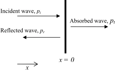
Incident wave, pi

Reflected wave, pr

Absorbed wave,pt

[image:19.595.237.431.81.199.2]

x = 0 x

Figure 2.1 Reflection of a sound wave incident normal to a surface

On incidence to a surface the energy of a plane wave is split into reflected and absorbed energies. The absorbed energy could be as a result of acoustic transmission though the surface or as heat conversion in the material. The proportion of energy that is not absorbed is reflected, this reflected wave will have both a different amplitude and phase from the incident wave such that the reflected wave can be given as:

( )

0

ˆ

, j t kx

r x t Rp e

p ₌ ω+

(2.1)

where R is the reflection factor of the surface. The reflection factor is a complex ratio of the reflected and incident pressures given by:

( )

x t p

t x p e R R

i r j

, ,

= = φ

(2.2) 2.2.2 Absorption Coefficient

(20)

To derive the absorption coefficient the intensity of a plane wave is considered as given by: c p I 0 2 ρ = (2.3)

Therefore on reflection, the reflected wave is reduced in intensity by a fraction of |R|2

and consequently the fraction of energy absorbed can be given by 1- |R|2. The absorption coefficient of a surface is therefore expressed as:

2

1− R

= α

(2.4)

The absorption coefficient of a material is probably the most widely used quantity when describing absorbent materials and systems and an absorber’s performance is often given by a graph of absorption coefficient versus frequency.

2.2.3 Surface Impedance

The surface impedance is a very useful parameter as it is very closely linked to the physical properties of a surface so it provides clear indication of how the surface behaves given an incident wave. The surface impedance is given by the ratio of pressure and the particle velocity normal to the surface:

) , ( ) , ( t x u t x p z= (2.5)

With the surface at x = 0 the combined pressure and velocity normal to the surface can be given by:

(

)

(21)

The surface impedance becomes:

R R c z

− + =

1 1

0

ρ

(2.7)

Separating the surface impedance into its real and imaginary components reveals information as to the magnitude of absorption and is resonant characteristics which can be very useful in analysis.

2.3 Porous Absorbers

When most people think of acoustic absorbers they commonly think of porous absorbers, this is because there are so many materials that are naturally porous and consequently absorb sound. Many people, in the pursuit of constructing a home studio or attempting some rudimentary acoustic treatment of an existing room, will use common materials such as thick curtains, carpets and sofa’s to control the reverberation time within the room, these all constitute porous absorbers. Porous absorbers must have open pores as in Figure 2.2 i.e. pores that can support acoustic propagation where the orifice is at the surface of the absorber. Porous absorbers can be either granular or fibrous providing they have these open pores. Granular absorbers can be made from small pieces of almost any rigid or semi rigid material bound together with glues that do not block pores. Loose granular materials such as sand also constitute porous absorbers as the gaps between grains provide a complex path for the acoustic waves to propagate through, but their loose nature often means they are impractical to use, especially in room acoustics. An example of a fibrous porous absorbent is mineral wool, made by spinning molten minerals such as sand and weaving the spun fibres together to form a complicated structure of pores. This complex pore structure leaves a material that is highly porous and is commonly used for both acoustic and fire insulation as its open pores allow restricted airflow through the material thus absorbing sound and also preventing efficient heat exchange.

(22)

porous absorbers making them efficient for room acoustic applications. For a porous absorber to be effective, it is important that the pores are open rather than closed. The diagram below shows the differences between closed and open cell foam:

a) b)

Figure 2.2 a) Closed cell foam, no propagation path through absorbent as pores are closed and

unconnected. b) Open celled foam, interconnected pores allow for acoustic propagation and consequent thermal/viscous losses. (From Cox and D’Antonio [8])

(23)

wavelength from the boundary). With this in mind it becomes clear that as the wavelength of the incident sound increases, the porous material must increase in depth if satisfactory absorption is to be achieved. This is the reason that porous absorption is unsuitable for treating low frequency modal problems in rooms, because the wavelengths are sufficiently large that much of the room would be taken up by the porous absorption, which is impractical. An exception to this is in the construction of anechoic chambers where broadband absorption is needed across the entire audio spectrum; porous absorption is used here so the absorption coefficient is roughly equal across a large bandwidth (a useful characteristic of porous absorption). Very thick porous absorption is used to tackle even the low frequencies in this case as low frequency resonant absorption would reflect and cause problems at higher frequencies.

2.3.1 Characterising and Modelling Porous Absorbers

It is often important to be able to predict accurately the performance of porous absorbers both for use on their own and also when used as part of a resonant absorber (see section 2.4). Being able to predict the reverberation time of a room and even to auralise its response before building or before acoustic treatment is added is becoming increasingly important in room acoustic design. With the increase in building regulations governing the acoustic insulation requirements of buildings, it is also imperative that the absorption characteristics of materials is known before building to ensure the building will reach the necessary standards on completion. This task is only possible when accurate information can be given about the absorption within the room. For these reasons and to aid research into the development of new absorptive materials much attention has been placed on defining the characteristics of materials and also predicting their acoustic performance. In order to accurately model porous materials it is important to determine certain physical properties of the material.

2.3.1.1 Material Properties

(24)

the material constitutes the air in the pores, the other half (the material that supports the pore structure) would be the ‘frame’ of the material. Closed pores do not count in measurements of porosity as they cannot be accessed by incident sound waves and are therefore ineffective for absorption. Foam with entirely closed pores would have a porosity of zero.

Flow resistivity is a metric that defines how easily air can enter a material and the resistance to flow that it experiences as it passes through, analogous to electrical resistivity. It is a measure of how much energy will be lost due to propagation through the pores. Flow resistivity can be defined as the resistance to flow per unit thickness of the material. The viscous resistance to air flow through a porous material causes a pressure drop across the material which at low frequencies is proportional to the flow velocity, U and thickness of the material, d. The ratio of this drop in pressure with the product of the flow velocity and material thickness gives the material’s flow resistivity:

Ud p

Δ = σ

(2.8)

The flow resistance of a material can also be useful and is given by multiplying the flow resistivity by the material thickness. However flow resistivity is more useful in the modeling of acoustic materials and is the property used throughout this thesis.

Both porosity and flow resistivity are very important factors but it is the flow resistivity that varies the most from material to material and therefore is considered the most important factor. The porosity of an effective porous absorbent is often very close to unity and varies very little with different materials.

(25)

absorber. Pore shape is difficult to define as materials often exhibit many pores with very different shapes and as such it is a difficult parameter to accurately define.

There are many different strategies for the modeling of porous materials using a variety of different approaches with varying degrees of complexity and overview of some of these can be found in [9]. The primary model used in this thesis is a one parameter empirical approach by Delany and Bazley [10]. In this model the porosity is considered to be unity and the material parameter needed is the flow resistivity. It is therefore important that the flow resistivity of the material used is accurately measured; the following describes the process of this measurement.

2.3.1.1.1 Measuring Flow Resistivity

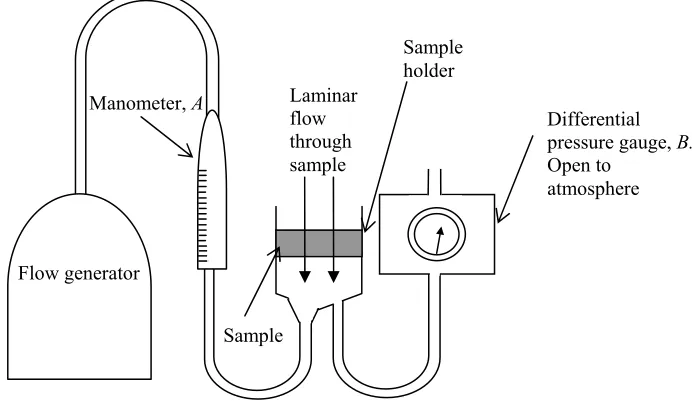
Flow resistivity can be measured using a relatively simple experimental setup as shown in Figure 2.3. The premise is to induce airflow through the test sample and to measure the resulting pressure difference across the sample. Details of this procedure are outlined in an international standard [11]. The standard outlines two different methods for the measurement of flow resistivity, the first utilising unidirectional airflow and the other an alternating airflow. The apparatus chosen here typified an apparatus to measure flow resistivity using unidirectional laminar flow.

Flow generator

Sample

Laminar flow through sample

Sample holder Manometer, A

Differential pressure gauge, B.

[image:25.595.153.499.505.710.2]

Open to atmosphere

(26)

In Figure 2.3 the manometer, A is used to calculate the airflow velocity through the sample, this is achieved in the test apparatus using the calibration chart for this particular set up which can be found in Appendix A. From this manometer reading the volumetric airflow rate, qv can be determined in cubic meters per second. When divided by area this gives the linear airflow velocity, V. The pressure difference across the sample with respect to the atmosphere can be deduced from the differential pressure gauge, B. from these values the specific airflow resistance, Rs can be written as:

V p q

pA R

v s

Δ = Δ

=

(2.9)

Where is the pressure drop across the sample measured with the differential pressure

gauge, and A is the cross sectional area of the sample. The flow resistivity σ of the sample is the specific flow resistance per meter:

p

Δ

Vd p d R_s ₌ Δ =

σ

(2.10)

where d is the depth of the sample.

This gives a measure of flow resistivity which can be used in many acoustic models and will be used in subsequent sections of this work in a basic one parameter model for rigid frame porous materials as part of a transfer matrix model presented later.

2.3.1.2 Prediction Models

(27)

techniques they then put an empirical formula together to allow the prediction of both the characteristic impedance and the complex wavenumber of fibrous absorbent materials. The formulae assume porosity close to unity and include the material’s flow resistivity, accurate only between 1000 and 50000 MKS raylm-1. Delany and Bazley’s is a single parameter model meaning only the material’s flow resistivity is needed for calculation. The model can be summed up in the following three equations. First they define a dimensionless variable X, dependent on the density of air within the pores ρ0, the frequency f and the flow resistivityσ:

σ

ρ f

X ₌ 0

(2.11)

Then the Characteristic Impedance zc and the complex wavenumber k are defined:

zc = ρ0c0(1 + 0.0571X-0.754 - j0.087X-0.732)

(2.12)

k = (ω/ c0)(1 + 0.0978X-0.700 - j0.189X-0.595)

(2.13)

(28)

2.3.1.2.1 Acoustic Impedance Modelling of Multiple Porous Layers

Often important in acoustic modeling and applications is the behaviour of acoustic waves propagating through layers of different media. This encapsulates many scenarios, ranging from sound traveling through a porous absorbent mounted on a rigid backing through to more complicated situations where there are many layers all with different characteristic impedances and the overall impedance needs to be found. In order to study accurately the behaviour of sound in these cases a modeling system needs to be formulated. Considering a wave approach enables a simple model to be put together, often called a two port model as it has just two ports (both a single input and single output). This type of model can also be extended to work for more complicated situations where further resonant layers are introduced (see section 2.4.2.1.1).

Considering plane waves incident only normal to the surface, a diagram of an acoustic wave incident to a multiple layered absorber can be represented by Figure 2.4:

d

x=− x=0

d pi

pt

pr

Medium A Medium B

x -direction

Figure 2.4 Diagram of sound propagation through multiple layers

At any point the total pressure can be seen as simple addition of the incident, reflected and transmitted pressures such that:

jkx r jkx i jkx t

t x pe pe p e

p ₍ ₎= − = − +

(2.14)

(29)

r i

t p p

p (0)= +

(2.15)

Velocity is a vector quantity therefore the addition of the velocities before and after the boundary of the layer is:

(

i r

)

c r i

t p p

z u u

u (0)= − = 1 −

(2.16)

where zcis the characteristic impedance of material A.

From equations 2.14 and 2.15, the incident and reflected pressures at the boundary can be expressed as:

0 = x c t i r c t r i z u p p z u p p ) 0 ( ) 0 ( − = + = (2.17) Therefore:

(

)

(

t t c

)

r c t t i z u p p z u p p ) 0 ( ) 0 ( 2 1 ) 0 ( ) 0 ( 2 1 − = + = (2.18)

So the sound pressure at any point x in space (assuming normal incidence) can be given by equation 2.19:

(

)

(

)

jkx

c t t jkx c t t jkx r jkx i

jkx _p _e _p _e _p _u _z _e _p _u _z _e

pe x

p (0) (0)

2 1 ) 0 ( ) 0 ( 2 1 ) ( = − = − + = + − + − (2.19)

(30)

(

)(

)

(

)(

) sin( ) 0 ( ) cos( ) 0 ( ) ( sin( ) cos( ) 0 ( ) 0 ( 2 1 ... sin( ) cos( ) 0 ( ) 0 ( 2 1 ) ( kx j u z kx p e p x p kx j kx z u p kx j kx z u p e p x p t c t jkx t t c t t c t t jkx t t − = = ⎥⎦ ⎤ ⎢⎣ ⎡ ₋ ₊ + ⎥⎦ ⎤ ⎢⎣ ⎡ ₊ ₋ = = − −

)

(2.20)

And the transmitted velocity as:

(

)

(

)

(

)

) sin( 1 ) cos( ) ( 2 1 2 1 1 1 ) ( kx j p z kx u e u x u e z u p e z u p z e p e p Zc e u x u t c t jkx t t jkx c t t jkx c t t c jkx r jkx i jkx t t − = = ⎥⎦ ⎤ ⎢⎣ ⎡ ₊ ₊ ₋ = − = = − − − − (2.21)

The ratio of the transmitted pressure and velocity at a point x gives the acoustic impedance at that point. So in order to find the impedance at the boundary of material A,

. Substituting this into the above equations gives:

d x=−

2

( ) (0) cos( ) (0)sin( )

( )

( ) _{(0) cos( )} _{(0)sin( )}

(0) cot( ) (0)

(0) cot( ) (0) cot( )

t t c t

t

t t

c

t c c t

t c t

t c c

t t c

p d p kd jz u kd

z d

j

u d _u _kd _p _k

z

jp z kd z u

ju z kd p

jz z kd z

z jz z kd

− + − = = − ₊ − + = − + − + = − d (2.22)

Where zt is the surface impedance at x=0(termination impedance) given by pt(0)/ut(0),

zc is the characteristic impedance of the layer with thickness d. zt(-d) is the surface impedance at the point x=−d. k is the wavenumber in the material, this can often be determined by a simple empirical model for porous absorbents or as 2πf /c if in air.

(31)

2.4 Resonant Absorption

Unlike porous absorption, which is used primarily for absorption of mid to high frequency sound, resonant absorption is most commonly used for treating low frequency acoustic problems. Resonant absorption is sometimes used for higher frequency applications where porous absorbers are impractical i.e. where weather or fumes could damage or clog the pores. It is however not common to use resonant absorption for higher frequency problems because the bandwidth of absorption is commonly a lot lower than porous absorption if high absorption coefficients are to be achieved. This narrow bandwidth corresponds to a very small fraction of an octave band at higher frequencies so is often considered impractical.

Resonant absorbers are essentially mass-spring systems where sound pressure incident on the absorber causes a mass element to vibrate on a spring which is damped to introduce energy loss and consequently absorption. Resonant absorbers are most efficient if placed in areas where acoustic pressures are high, as higher pressures induce greater movement of the mass. As a result, resonant absorbers are often placed on the boundaries of a room and often in the corners where room modes have maximum pressure amplitude so maximally efficient absorption can be achieved. This contrasts with porous absorbers, which are most effective in areas of maximum particle velocity i.e. away from boundaries.

There are two main types of resonant absorption, namely Helmholtz absorbers named after Hermmann Von Helmholtz (1821-1894) and membrane absorbers. Both are commonly used in room applications and also as silencers in engines and ventilation ducts et cetera. Theory of both techniques is presented in the following sections.

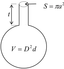
2.4.1 Helmholtz Absorbers

Helmholtz absorbers consist of a plate with many holes equally spaced in both the x and

(32)

Resonant air flow

[image:32.595.148.256.577.693.2]

through perforations _D

Figure 2.5 Schematic representation of a typical Helmholtz absorber

Both membrane and Helmholtz resonant absorption attempt to convert areas of high acoustic pressure into a region of high particle velocity that can be absorbed by intelligently positioned porous absorption. In the case of a Helmholtz absorber, incident pressure causes highest particle velocity in the neck of each orifice so porous materials are often placed there to maximise absorption efficiency, in practical applications however the porous absorbent is usually placed in between the two plates for ease of manufacture and cost efficiency.

2.4.1.1 Predicting the Performance of Helmholtz Absorbers

The performance and resonant frequency of Helmholtz absorbers is easy to predict and can be done to a high degree of accuracy by considering each orifice to be a short tube forming individual Helmholtz resonators as shown in Figure 2.6:

Figure 2.6 Diagram of a Helmholtz type acoustic resonator

Porous Absorbent

Sealed

enclosure Perforated sheet

2a t

d

d D V ₌ 2

2

a S =π

(33)

A short tube terminated with a low impedance behaves like an inert mass, [7] therefore the acoustic mass per unit area of the Helmholtz absorber is given by equation 2.23

assuming the geometry given in Figure 2.5:

ε ρ π

ρ t

a t D

m 0

2 2

0 ₌

=

(2.23)

where ₂2

D a

π

ε = and is termed the fractional open area or ‘porosity’ of the perforated

sheet.

Each plug of air is considered to behave like a baffled piston such that it is subject to a radiation impedance given by equation 5.19, [15]. The value of this radiation impedance depends on whether or not the holes are flanged. Considering a flanged termination introduces an end correction as a result of the radiation impedance which adds an apparent extra length of 8a/3π ≈0.85a to each end of the plug of air thus equation 2.23

becomes:

ε ρ ε

ρ₀(t 1.7a) ₀t'

m= + =

(2.24)

where is the apparent length of each plug as a result of end corrections. The mechanical impedance of a Helmholtz resonator is the sum of the impedance due to radiation resistance Rr, stiffness K, and mass per unit area m, such that:

t′

r

M R

j K m j

Z = + +

ω ω

(2.25)

Considering just one plug, ε becomes unity and the stiffness of the plug can be expressed as [15]:

V S c K

2 2 0

ρ =

(34)

The resonant frequency can therefore be determined by setting the imaginary part to zero. The resonant frequency can then be found by:

(

)

' 2 ' 2

' / 2

1

0

0 2 2 0 0

dt c Vt

S c f

t V s c f

ε π π

ρ ρ π

= =

=

(2.27)

To formulate the absorption of a Helmholtz absorber it is possible to define a lumped element model as in chapter 5, it is often more helpful however to consider in the entire acoustic system as a combination of layers as part of a transfer matrix model (see section 2.4.2.1.1). In this case the impedance of the perforated sheet is simply added onto the impedance of the backing to find the overall impedance; from here the absorption coefficient can easily be found from equations 2.7 and 2.4.

2.4.2 Membrane Absorbers

Membrane or panel absorbers are also mass-spring systems, this time however the vibrating mass is a flexible membrane or plate and the spring is the compliance of the sealed air cavity of the box backing the membrane. A standard design of membrane absorber is shown below:

Porous Absorbent Particle velocity v

Movement of membrane

Small gap to allow free movement of membrane/panel

Enclosure, with

compliance C Flexible membrane/panel Mass/unit area m

Figure 2.7 Schematic representation of a standard membrane absorber

(35)

the fundamental frequency range, which is almost always the case with membrane absorbers. The vibration of the membrane creates high particle velocities at its rear that effectively force air through the porous absorbent thus generating high levels of absorption. This however is only over a limited bandwidth i.e. the resonance peak of absorption has a high Q-factor. The bandwidth can be increased by increasing the damping, but as with any mass-spring system, this has the effect of decreasing the maximum efficiency of the absorber. A trade off therefore ensues between bandwidth and maximum absorption.

Unlike Helmholtz absorbers, prediction of the behavior of membrane absorbers is difficult and often inaccurate this is because the exact mounting conditions and properties of the membrane are hard to predict and model. Not being able to model the mounting conditions accurately is problematic as membrane absorbers often exhibit losses and hence absorption from the edges. Many common formulations also assume that the membrane cannot support higher order modes than the fundamental resonant frequency i.e. they assume that the membrane moves as a lumped mass system in much the same way as a piston does. These simpler models do not allow for the membrane to support bending waves and consequently don’t result in accurate predictions especially at oblique incidence, when bending waves are more easily excited.

2.4.2.1 Predicting the Performance of Membrane Absorbers

If the membrane is considered to oscillate as a piston and its bending stiffness is ignored such that the restoring force is entirely due to the compliance per unit area C of the air volume where:

2 0c

d C

ρ =

(2.28)

An equation of the impedance of the cavity backed membrane can then be written as:

M R C M j

Z ⎟+

⎠ ⎞ ⎜

⎝

⎛ ₋

=

ω

ω 1

(36)

where M is the mass per unit area of the membrane or plate and RM is the mechanical losses of the mounting. The resonant frequency of this system can be found by setting the imaginary part to zero thus:

2 1 2 0

0 ⎟⎟

⎠ ⎞ ⎜⎜ ⎝ ⎛ =

Md c

ρ

ω , so

Md f₀ ≈ 60

(2.30)

Equation 2.30 is a useful first approximation but it only defines the condition with an empty cavity. If the cavity contains porous absorbent as is common in the design of such absorbers the resonant frequencies predicted by this formula tend to be too high. This formula can therefore be altered to account for the adiabatic case as [7]:

Md f₀ = 50

(2.31)

These provide a useful first approximation but often yield inaccurate results with errors of up to 10 per cent. This inaccuracy is largely because the mechanical properties of the panel are not taken into account. With the edges of the panel fixed its bending stiffness will, especially for thicker panels, contribute considerably to the restoring force of the system such that it cannot be approximated simply by equation 2.28. Accurately predicting this bending stiffness is particularly difficult especially when the exact boundary conditions of the membrane or plate are uncertain.

16,17

(37)

2.4.2.1.1 Transfer Matrix Modelling

The transfer matrix approach is a very useful tool as it allows surface velocities, pressures to be calculated this enables the more useful determination of the surface impedance.

Writing equation 2.22 in matrix form gives the pressure and velocity at a point x as:

⎭ ⎬ ⎫ ⎩ ⎨ ⎧ ⎪⎭ ⎪ ⎬ ⎫ ⎪⎩ ⎪ ⎨ ⎧ = ⎭ ⎬ ⎫ ⎩ ⎨ ⎧ ) 0 ( ) 0 ( ) cos( ) sin( ) sin( ) cos( ) ( ) ( t t c c t t u p kd kd z j kd jz kd x u x p (2.32)

This is part of a transfer matrix that can be found in Allard [14]. The transfer matrix method uses the surface impedance of one layer as the backing impedance of the next enabling any number of layers to be combined and the final surface impedance found. It is a very useful tool for designing absorbers as it eliminates the need for iterative development which is both costly and time consuming in the design of absorber systems. The transfer matrix method allows many different systems to be predicted ranging from the simple case of a porous material mounted on a rigid wall up to multiple porous layers including membrane and Helmholtz layers. In order to perform calculations, the characteristic impedance of the material of each layer must be known. This can be achieved easily in many cases such that a porous layer can be represented by empirical or semi-empirical formulations like the Delany and Bazley model as mentioned in section 2.3.1.1. The characteristic impedance of membrane and Helmholtz layers can be more problematic to predict with accuracy as often boundary conditions are not known and as such approximations have to be made. For the membrane case the membrane is assumed to be very thin such that there are no bending waves present. It is thereby assumed to move as a pistonic mass. The impedance in this case can be considered as a series combination (that is the simple addition) of a single resistive and reactive term. In general membranes are assumed to move pistonically with a nominal resistance to motion made up from the mounting and resistive losses in the material. The impedance therefore is given by equation 2.35.

(38)

[image:38.595.120.568.135.484.2]

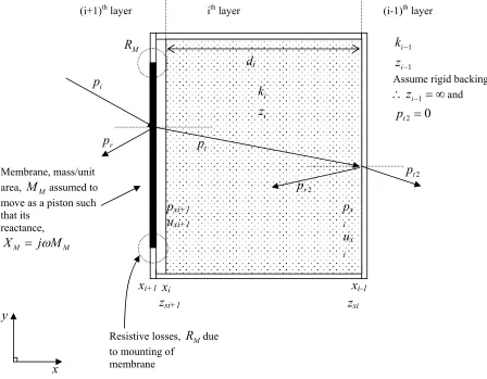
system can be represented by Figure 2.8. The initial case is considered with a membrane mounted on a cabinet filled with absorbent material.

Figure 2.8 Diagrammatic representation of the transfer matrix modeling of sound incident to a membrane

absorber

The equation that links all of the surface pressures and velocities and allows hence the calculation of the surface impedance is the same as in section 2.3.1.2.1 but with different notation equation 2.22 can therefore be written as:

( )

i i i si i i i i si si d k jz z z d k z jz z cot cot 2 1 ₋ + − = + (2.33) r p i p

(i+1)th_layer _ith_layer _(i-1)th_layer

1 1 − − i i z k t p 2 r

p t2

p M

R

di

Assume rigid backing:

i i z

k _∴ ₋ ₌_∞

1 i z and 0 2 = t p Membrane, mass/unit area, assumed to move as a piston such that its reactance, M M j _M M M

X = ω

Resistive losses, due to mounting of

m M R embrane pxi+1 uxi+1 px i ux i

xi+1 xi xi-1

zsi+1 zsi

y

(39)

Using this notation it easier to keep track of multiple layered systems. Applying this to the ith layer, the backing is considered to have infinite impedance such that z_si ≈∞and the above equation simplifies to:

) cot(

1 i i i

si jz kd z ₊ =−

(2.34)

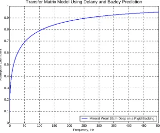
Where ki can be determined from a model for porous media such as Delany and Bazley and di is the depth of the porous material. This value can then be used as zsi for the next layer and the impedance calculated for further layers of materials. From this the absorption coefficient can be calculated and plotted against frequency yielding the standard result for mineral wool as shown in Figure 2.9:

1

0 50 100 150 200 250 300 350 400 450

0.9

0.8

0.7

0.6

0.5

0.4

0.3

0.2

0.1

500 0

Frequency, Hz

A

bs

orpt

ion C

oef

fi

c

ient

Transfer Matrix Model Using Delany and Bazley Prediction

[image:39.595.145.475.338.614.2]

Mineral Wool 10cm Deep on a Rigid Backing

Figure 2.9 Transfer matrix modeling of porous absorbent with a rigid backing using the Delany and

Bazley model

(40)

M M

M j M R

z = ω +

(2.35)

The surface impedance of the system is then the series addition of the impedance of the membrane layer and the porous layer:

M si si z z z ₊₁ = +

(2.36)

More complex solutions can be obtained if air gaps and/or Helmholtz layers are included, for now the simplest case is considered as shown in Figure 2.8 with a membrane layer added to the porous absorbent with a small air gap between the layers to allow for the membrane’s movement. Plotting this in MATLAB yields the prediction in Figure 2.10:

1

0 50 100 150 200 250 300 350 400 450

0.9

0.8

0.7

0.6

0.5

0.4

0.3

0.2

0.1

0

500 Frequency, Hz

A

bs

orpt

ion C

oef

fi

c

ient

Transfer Matrix Model of Simple Membrane Absorber System

Figure 2.10 Transfer matrix prediction of a simple membrane absorber

(41)

The predictions so far have dealt only with waves incident normal to the surface of an absorber, this is a useful case and matches closely to the testing of an absorber in an impedance tube and therefore is very useful for comparison of predictions and measurements. There is however scope for extending the transfer matrix approach for oblique incidence waves by considering the wavenumber in materials as a vector quantity with components in the x and y direction. Such that:

2 2 2

y x k k + = k

(2.37)

Using Snell’s law it is then possible to define the refractive effect as the acoustic waves propagate through each medium. The equation then becomes:

(

)

(

xi i

)

xi i si

xi i i i xi xi

i i si si

d k k

ki jz z

k k z d k k

k z jz z

cot cot

2

1

−

⎟⎟ ⎠ ⎞ ⎜⎜ ⎝ ⎛ + −

= +

(2.38)

For most porous absorbents the x component of the wavenumber vector, k is equal to the scalar wavenumber in that material as the angle of incidence tends to the normal. Thus often the angle of incidence is not needed. For the purposes of this project only normal incidence will be modeled.

2.5 Conclusion

(42)

3. MEASURING ABSORPTION

COEFFICIENT AND SURFACE

IMPEDANCE

3.1 Introduction

The previous chapter outlined some theory and prediction techniques for the performance of acoustic absorbers. This chapter describes and demonstrates some useful techniques for the measurement of absorption characteristics. Of primary interest is the surface impedance of an absorber, be it porous or resonant. From this quantity, the reflection factor and the absorption coefficient can be found giving a good idea of the absorber’s performance with respect to frequency.

(43)

used to test larger areas of absorbers such as carpets where samples with large surface area can easily be obtained. Impedance tubes require much smaller samples and are often used when developing new absorbers as small samples are more cost effective to produce. The normal incidence absorption coefficient measured in this case is also easier to compare with theoretical models than the random incidence absorption coefficient which is very difficult to predict so is less useful for comparisons.

Both techniques are presented in this chapter along with the design, construction and commissioning of a low frequency impedance tube especially designed for the measurement of low frequency absorbers. The cross sectional area of the tube was such that the entire membrane absorber could fit into it thus allowing accurate testing of its normal incidence absorption coefficient.

3.2 Reverberation Chamber Method

The basic premise of the reverberation method is to determine how much difference an absorber makes to the reverberation time in a room, and therefore to determine the absorption coefficient of the material that would result in this difference. The reverberation time is measured before and after the addition of the absorption and from this, the absorption coefficient is derived. The reverberation chamber method is based on Sabine’s equation for the reverberation time in a room [18]:

cA V T =55.3

(3.1)

Where T is the time for the noise source within the room to decay by 60dB from a steady level, V is the volume of the room, c is the speed of sound and A is the total absorption area of all surfaces. Rearranging this formula and adding a term for the absorption due to the air (this becomes significant for larger rooms) gives an equation for the equivalent sound absorption area of the empty reverberation room, A1:

1 1

1 4

3 . 55

m cT

V

A = −

(44)

The equation for the equivalent sound absorption area of the reverberation room with the absorption present, A2 is then given by:

2 2

2 4

3 . 55

m cT

V

A = −

(3.3)

where T1 and T2 are the reverberation times and m1 and m2, the power attenuation coefficients of the room, without and with the sample respectively. Combining these equations gives a formula for the equivalent sound absorption area of the sample as follows:

(

2 1

)

1 1 2 2 1

2 4

1 1 3 .

55 V m m

T c T c V A

A

A_T _⎟⎟− −

⎠ ⎞ ⎜⎜

⎝ ⎛

− =

−

=

(3.4)

The random incidence absorption coefficient of the test sample can then be easily calculated by:

S A_T s =

α

(3.5)

A more detailed description of this method can be found in an international standard [19]. The random incidence absorption coefficient measured by the reverberation chamber method is more true to life than the normal incidence coefficient as sound is commonly incident to a surface from all angles so this method can be useful to see how absorbers behave in real applications like determining how much sound energy a carpet will absorb if used in a domestic setting. Consequently it is the random incidence absorption coefficient that is most commonly used to define the performance of materials used in architectural acoustics. A disadvantage of this method is that it doesn’t allow the impedance of the material to be measured which prevents a complete understanding of how the material behaves acoustically. Further to this, the method requires a reverberation chamber and large samples so it can be expensive to undertake.

(45)

impedance tube method outlined in section 3.3 that is used for measurements throughout this work.

3.3 Impedance Tube Method

Impedance tubes offer a more controlled test environment and have the advantage over the reverberation method that they enable the measurement of the acoustic impedance of a sample or system. Impedance tubes are cheaper to use than the reverberation chamber technique because less specialist equipment is needed; also the sample sizes can be much smaller, cutting down on waste. There are two techniques for using impedance tube; the standing wave method and the transfer function or ‘two-microphone method’. Both methods are outlined below and can also be found in the relevant International Standards [20, 21]. Brief theory of both methods is given below.

3.3.1 Standing Wave Method

The standing wave method was the earliest method devised for measuring absorption using a tube it evolved from August Kundt’s (1839-1894) tube for measuring the speed of sound and is simpler in principle than the transfer function approach. The basic premise is as follows. Plane waves propagate down the tube from the loudspeaker and are reflected from the other end of the tube where the sample is mounted, consequently setting up standing waves in the tube. Measuring the relative amplitudes of the maxima and minima of the standing waves using a moving probe microphone enables the absorption coefficient to be calculated, for discrete frequencies. A diagram showing the construction and operation of a standing wave tube is shown in

Figure 3.1:

Figure 3.1 Diagram of the typical setup of an impedance tube using the standing wave method

With the loudspeaker source on, a standing wave will be set up in the tube. The probe microphone can be moved up and down the tube in order to find the first pressure maximum and the first pressure minimum from the sample. This can be done by simply connecting the output from the microphone to a voltmeter. Noting down the values and

Rigid Termination Probe Tube

Microphone

Trolley

Loudspeaker

(46)

their position relative to the sample allow for both magnitude and phase data to be determined and used to calculate the absorption coefficient and the surface impedance of the sample. As this procedure has to be done separately for each frequency of interest it can be rather time consuming and doesn’t give continuous data. It is however a reliable method and simple equations can be used to calculate the necessary parameters of the sample as shown below.

The pressure at any point in the tube, assuming plane wave propagation, will be given by:

r i p p

p= +

(3.6)

where pi = Aejkz and pr = ARe-jkz. Therefore:

p = A(ejkz + Re-jkz)

(3.7) z is the distance from the sample, k is the wavenumber, R is the reflection factor and A is a complex constant. For a pressure maximum the incident and reflected waves interfere constructively and are therefore in phase. For a pressure minimum the incident and reflected waves interfere destructively and are therefore 180 degrees out of phase, therefore equations for pmax and pmin can be given as follows:

pmax = 1 + |R| pmin = 1 - |R|

(3.8)

Knowing only the magnitudes of pmax and pmin the reflection factor can be calculated by finding the standing wave ratio (SWR) between the two pressures.

R R p

p SWR

− + = =

1 1

min

max

(3.9)

⇒

1 1 + − =

SWR SWR

Improved membrane absorbers