Simulation of Electromagnetic Field Distribution in Metallic Waveguides Using Open Source Finite Element Software

(1)

International Journal of Emerging Technology and Advanced Engineering

Website: www.ijetae.com (ISSN 2250-2459,ISO 9001:2008 Certified Journal, Volume 3, Issue 2, February 2013)

91

Simulation of Electromagnetic Field Distribution in Metallic

Waveguides Using Open Source Finite Element Software

Ndagije Charles

1

, Geuzaine Christophe

2

1_{Faculty of applied sciences, National University of Rwanda, P.O. Box 117 Butare (Rwanda).} 2_{University of Liège, Institut Montefiore (B28), B-4000 Liège (Belgium)}

Abstract- Computer simulations and modeling of physical processes can play an important role in teaching engineering courses, in particular for difficult courses like electromagnetic and microwave engineering. In this paper we analyze the mode distribution in metallic waveguides by using open source finite element software from the OneLab project: Gmsh and GetDP. The resulting fully parameterized finite element models have been used in teaching the course of microwave communication at the National University of Rwanda and have played an important role to facilitate the students’ understanding of the course.

Keywords- Maxwell’s equations, waveguide, finite element method, electromagnetic field, weak formulation, discrete formulation, Galerkin Method.

I. INTRODUCTION

Many universities, especially those in developing countries, suffer from the lack of (often expensive) laboratory equipment for conducting practical courses on important engineering topics, like electromagnetic and microwave engineering. One way to improve the manner those courses are taught is to use simulation techniques.

Modeling and simulation can help students to better understand such courses without using hardware equipment. In addition, successful modeling and simulation requires a very good understanding of the subject, some mathematical knowledge and computer skills which all contribute to the overall training of engineering students. Many physical phenomena and processes can be described by differential equations that are often hard or impossible to solve analytically, which complicates their analysis. In this paper we propose to set up parametric finite element models to compute the distribution of electromagnetic fields in metallic waveguides. Such metallic waveguide are widely used in telecommunication for ultrahigh and super high frequencies. Modeling such waveguides requires the solution of Maxwell’s equations, which can be obtained numerically by using the finite element method [11].

We propose to evaluate both the time-dependent and time-harmonic solution of Maxwell’s equations in these waveguides, as well as the eigenvalues which are in our case the operating frequencies for a considered mode.

The main advantages of using the finite element method for analyzing the wave propagation in the waveguides is that it makes it easy to determine the operating frequency for arbitrary geometries, while by using analytical methods it is only possible to determine the critical frequency and the condition for which the wave can be able to propagate for simple geometrical configurations.

In the context of engineering courses such numerical simulations can help to clearly display wave patterns and other relevant physical quantities (e.g. S matrix) without using laboratory equipment. In addition, by building fully parameterized models (where the dimensions, materials, operating frequency, …, can be changed interactively) the simulations can help to understand experimental measurements and to design new applications.

The results of this work have been used in teaching the course of microwave communication at the National University of Rwanda in 2010 and 2011 to the population of about 50 students. The developed parametric models helped the students to easily understand that by changing the parameters of the wave guide the operating frequencies are also changing as well as the distributions of corresponding modes in waveguide.

All the models were prepared using the open source finite element tools from the OneLab project, in particular the GetDP and Gmsh codes developed by the team of Professor Christophe Geuzaine at the University of Liège in Belgium [1]. Since the software tools are freely available on the internet, both students and Faculty can use them without restrictions.

(2)

International Journal of Emerging Technology and Advanced Engineering

[image:2.612.54.282.166.303.2]

92

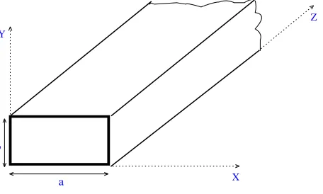
Let start by analyzing simple rectangular waveguide invariant along the Z axis (see Figure 1).

Figure 1. Geometric representation of a metallic rectangular waveguide

Maxwell’s equations in linear media read:

. ,

. 0,

(1) ,

,

E

B

H E

t E

H j

t









 

      

 

   















Where

E

is the electrical field intensity ,



is the electrical charge density, B is magnetic flux density,



is the permeability of the medium,

H

is the magnetic field intensity, j is the conduction current density,



is the permittivity of the medium. If the considered medium is the air, the permittivity becomes



₀, and the permeability becomes



₀,where



₀



8,854.10



12 farad m

/

and

7 4 .10

/

0 henry m









.

By using the properties of vector analysis the system (1) of first order partial differential equations (PDEs) can be rewritten as the following second order equation:

2 0 0

2

0 E

dj

E

dt

t

 





 

 



(2)

In general the current density

j



is a function of time and space. In the cases that we are going to treat next we will assume that the metallic surfaces of the waveguide are perfect conductors;

j



will thus represent only a source of

the electromagnetic waves. The electrical field

E



must satisfy the boundary conditions, i.e., its tangential components must be equal to zero on the waveguide surfaces, meaning that the following condition has to be satisfied [5]:

0 n E

 

, where

n



is the outgoing unit normal vector. For effective transmission of information in waveguide it is very important to know if the transmission channel is adequate referring to the frequency to transmit. In order to know which waves (modes) are able to propagate through a given wave guide, we need to compute the eigenfrequencies

f Hz

[

]

of the guide. This problem can be solved by using finite element method.

III. FINITE ELEMENT METHOD

The finite element method is a computational technique which can help to approximate solutions to PDEs encountered in scientific and engineering applications [10].

With the finite element method the solution of PDEs is found by following different steps. The first step is the preprocessing which includes the definition of the geometric domain of the problem, the definition of elements type to use for domain discretization, the definition of material properties of the elements, and the definition of the physical constraints. The second step is the solution phase. During this step the finite element software assembles the governing algebraic equations in matrix form and computes the unknown values. This step requires the discrete formulation of the problem through the weak formulation of the problem (see section 5). For the discrete formulation of the problem we used the Galerkin method [10], [7] as implemented in the open source software GetDP [2].

The last step of finite element method is the post processing which is focused on analysis and evaluation of the solution results. In this study this step was carried out by using the Gmsh open source software [1].

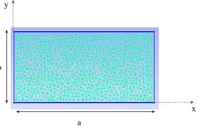
The next figure represents the discretization of the domain of resolution which is the cross section of the waveguide.

X Y

Z

b

(3)

International Journal of Emerging Technology and Advanced Engineering

[image:3.612.66.270.137.268.2]

93

Figure 2. Discretized cross section of the waveguide

IV. WEAK FORMULATION OF THE PROBLEM For the weak formulation of the problem, we used the method of weighted residual [10]. According to this method, instead of solving (2) directly, we look for

E



such that

2

. 0 (3) 0 0 2 0

E j

E U d

t t                      

  holds

for appropriately chosen weight functions

U

. By using the properties of vector analysis the equation (4) can be rewritten as follows:

2

.( ) . .

0 0 2

. 0 (4) 0

E

U A d U A d U d

t j U d t     _  _  _                               

Where

A

 

E

. The expression (5) becomes



(5) 0 . . ) ( ). ( ) ( ). ( 0 2 2 0 0                                  d U t j d U t E d U E d n A U              

To get the expression (6), it was considered that

(UA)n d (  ) U n.( A d) () (6)



 

Where





is a curve delimiting the surface



.

The term

A n U d

.(



) (

 

)

0 



, because it is

necessary to chose the weight function which also satisfies the boundary conditions such that

n U

 

0

.

Finally the integral in (4) can be written as follows:

. (7) 0 . . ) ( ).

( 2 0

2

0

0  

                       d U t i d U t E d U E           

This expression represents the weak formulation of the problem.

V. DISCRETE FORMULATION OF THE PROBLEM The discrete formulation consists in approximating the electric field

E

using a finite number of shape functions (basis functions)

_{W j}

:

1 (8) .

N

E

C W

_j

j

 



The GetDP code uses co-called Whitney edge elements to approximate the electric field. In this case, the functions

W j

have continuous tangential components across element borders, but discontinuous normal components and the coefficients

_{C j}

are the circulations of

E

along each

edge of the mesh.

N

is the total number of edges in the mesh. By using the Galerkin method, the weight functions

U

are chosen identical to has the shape functions, i.e.,

,

1, 2, 3,... (9)

k

U



W

k



N

.

Introducing (9) and (10) into (7) leads to a system of N linear equations:

2

. _{0 0}

2

1 1

0 0

j

N k j N W k

C_j Curl W Curl W d C_j W d

j j t

(4)

International Journal of Emerging Technology and Advanced Engineering

94

 (10)

0 2 0 0 . 1                                d k W t j d k W t i W d i W Curl k W Curl N

i Ci

        

The expression (10) is the discrete formulation of the problem. In this equation the unknowns are the values

C

_j The numerical resolution aims to find those values. Once they are found the electrical field

E



can be obtain by using the expression (8).

VI. NUMERICAL SOLUTION

We tested the method by solving the following eigenvalue problem derived from (10) with a zero source current:

 (11)

1 0 2 0 0          N j d k W j W d k W Curl j W Curl j

C       

Where



is the angular frequency (





2 

f

).

We first tested the case of TM-modes in 2D where we considered that _Ez is normal to the domain of study. For the second case, we considered the TE-modes, where the component _{H z}is normal to the 2D domain of study. The two considered modes differ by their boundary conditions. For TM-mode we used homogeneous Dirichlet boundary condition while for TE-mode we used the Neuman boundary condition.

[image:4.612.331.570.174.400.2]

A. TM- Modes

Table 1 shows that the values of critical frequency found by using finite element method is almost identical to that found by using the following analytical formula:

2

2 (12)

2 c

m

n

fc

a

b



 

_{ }



 

_{ }

 

Where

c

is the speed of electromagnetic wave in free space,

m

the number of the half wavelength along the width

a

, and

n

the number of the half wavelength along the height

b

.

TABLE I

COMPARISON OF CRITICAL FREQUENCY WITH EIGENFREQUENCY IN CASE OF TM-MODE

Mode type _{Eigenfrequency}

_f

(Hz)

Critical frequency

f

_c (Hz)

11

TM

1.677e+9 1.677e+9

21

TM

2.121e+9 2.121e+9

31

TM

2.704e+9 2.704e+9

12

TM

3.0927e+9 3.092e+9

13

TM

4.563e+9 4.562e+9

41

TM

3.355e+9 3.354e+9

32

TM

3.751e+9 3.75e+9

51

TM

4.0397e+9 4.039e+9

42

TM

4.244e+9 4.243e+9

13

TM

4.567 e+9 4.562 e+9

The electromagnetic wave will be able to propagate in a given waveguide only if its frequency is greater than or equal to the critical frequency. In the TM- case, the mode for which mn0 does not exist.

For numerical solutions, we used

a



0.2[ ]

m

and

0.1[ ]

b



m

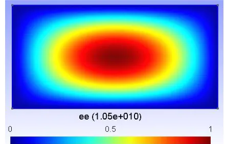
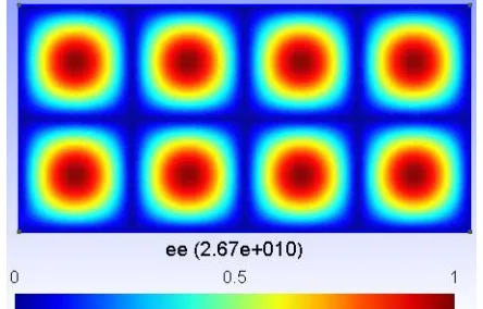
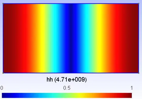
. Figures 3.1-3.8 show the norm of the electric field for the first few TM-modes. The numbers

n

and

m

are both different from zero.

[image:4.612.332.552.522.663.2]

(5)

International Journal of Emerging Technology and Advanced Engineering

95

[image:5.612.57.279.136.276.2]

Figure3.2: Norm of TM21-mode in the cross section of the waveguide.

[image:5.612.333.557.307.451.2]

Figure 3.3: Norm of TM31-mode in the cross section of the waveguide

Figure 3.4: Norm of TM12-mode in the cross section of the waveguide.

Figure 3.5: Norm of TM32-mode in the cross section of the waveguide.

[image:5.612.333.555.479.621.2]

(6)

International Journal of Emerging Technology and Advanced Engineering

96

[image:6.612.59.276.125.280.2]

Figure 3.9 illustrates the pattern of the vector field

H

.

Figure 3.9: Representation of

H

for TM11-mode

B: TE-Modes

The distribution of the electrical field for TE-modes in the cross section is found in a similar way , but by solving the following equations

2

0 0 0

2 (13)

0 ,

1

0 H

H

t

i

_{H z}

Ex

y

c

i

_{H z}

E

_x

i

x

c

 

 



   









 















instead of (2).

Table 2 compares the numerically obtained eigenvalues with the analytical critical frequencies for the first few modes. The two lowest critical frequencies are

10 TE

and

20 TE

.

TABLE II

COMPARISON OF CRITICAL FREQUENCY WITH THE EIGENFREQUENCY FOR THE CASE OF TE-MODES

Mode type

Eigenfrequency

f

(Hz)

Critical frequency

f

_c (Hz)

10

TE

7.504e+8 7.5e+8

01

TE

1.5027e+9 1.5e+9

20

TE

1.5016e+9 1.5 e+9

11

TE

1.678e+9 1.677e+9

21

TE

2.125e+9 2.121e+9

30

TE

2.255e+9 2.25e+9

31

TE

2.715 e+9 2.704e+9

40

TE

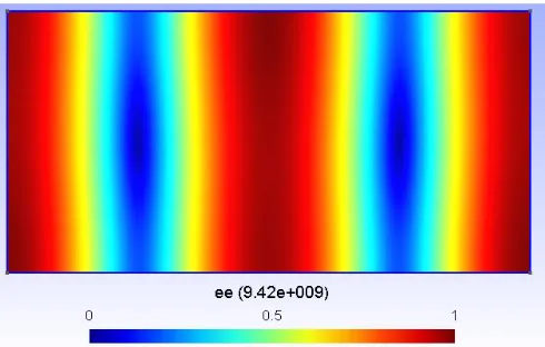
3.0022e+9 3 e+9

[image:6.612.49.289.311.487.2]

Figures 4.1-4.8 show the norm of the magnetic field for the first few TE-modes.

[image:6.612.325.570.476.648.2]

(7)

International Journal of Emerging Technology and Advanced Engineering

97

Figure4.2: Norm of TE20-mode in the cross section of the waveguide

Fig4.3: Norm of TE01-mode in the cross section of the waveguide

Fig4.4: Norm of TE11-mode in the cross section of thewaveguide

[image:7.612.46.572.58.693.2]

Figure 4.5: Norm of TE21-mode in the cross section of the waveguide

[image:7.612.50.295.133.289.2]

(8)

International Journal of Emerging Technology and Advanced Engineering

[image:8.612.51.295.123.283.2]

98

Figure 4.9 illustrates the pattern of the vector field

E



.

Figure 4.9: Representation of

E



for TE10-mode

VII. CONCLUSION

In this study the distribution of electromagnetic fields in the cross section of metallic rectangular waveguides has been described and simulated, by using the finite element method.

The found results were applied during the teaching of the course of microwave communication in third year electronics and communication systems at National University of Rwanda.

It was demonstrated that the simulation techniques can facilitate the better understanding of engineering courses. One of the particular advantages of finite element method is visualization of results which are sometimes an abstract concept.

Future work will explore the use of this methodology to study more complicated configurations, as well the dynamic propagation of electromagnetic fields in the time domain.

REFERENCES

[1 ] C. Geuzaine and J.-F. Remacle, Gmsh: a three- dimensional finite element meshes generation with built-in pre-and post-processing facilities. International for Numerical Method in Engineering, Volume 79, Issue 11, pages 1909-1331, 2009. http://www.geuz.org/gmsh.

[2 ] Patrick Dular, Christophe Geuzaine, A general environment for the treatment of Discrete Problems, University of Liege , 1997-2011. http://www.geuz.org/gmsh.

[3 ] Granino A. KORN, Advanced dynamic –System simulation, Willey & Sons, Inc., Arizona, 2007.

[4 ] W. J. Minkowycz, E. M.Sparrow, J.Y. Murthy, Handbook of Numerical heat transfer, second edition, Willey &Sons, Inc., United States of America, 2006.

[5 ] Robert E. Collin, Foundations for Microwave Engineering, second edition, John Willey &Sons, Inc., New York, 2001.

[6 ] G.R. Liu, S. S. Quek, The finite element method: A Practical course, Elsevier Science Ltd, Singapore, 2003.

[7 ] J.N. Reddy, An introduction to the finite element method, second edition, McGraw-Hill, In., Texas, 1993.

[8 ] Jean-Philippe Grivet, Méthodes numériques appliquées pour le scientifique et l’ingénieur, EDP Sciences, Paris 2009.

[9 ] Benoît Meys, Modélisation des champs électromagnétiques aux hyperfréquences par la méthode des éléments finis. Application au problème du chauffage diélectrique, Thèse présentée à la Faculté des sciences Appliquées, Université de Liège, 1999.

[10 ]David V. Hutton, Fundamental of finite element analysis, McGraw- Hill, New York, 2004.

[image:8.612.47.290.318.494.2]