Study on Coal Consumption Curve Fitting of the Thermal Power Based on Genetic Algorithm

(1)

http://dx.doi.org/10.4236/jpee.2015.34058

Study on Coal Consumption Curve Fitting

of the Thermal Power Based on

Genetic Algorithm

Le-Le Cui, Yang-Fan Li, Pan Long

State Grid MianYang Electric Power Supply Company, MianYang, Sichuan, China Email: [email protected], [email protected]

Received January 2015

Abstract

Coal consumption curve of the thermal power plant can reflect the function relationship between the coal consumption of unit and load, which plays a key role for research on unit economic oper-ation and load optimal dispatch. Now get coal consumption curve is generally obtained by least square method, but which are static curve and these curves remain unchanged for a long time, and make them are incompatible with the actual operation situation of the unit. Furthermore, coal consumption has the characteristics of typical nonlinear and time varying, sometimes the least square method does not work for nonlinear complex problems. For these problems, a method of coal consumption curve fitting of the thermal power plant units based on genetic algorithm is proposed. The residual analysis method is used for data detection; quadratic function is employed to the objective function; appropriate parameters such as initial population size, crossover rate and mutation rate are set; the unit’s actual coal consumption curves are fitted, and comparing the proposed method with least squares method, the results indicate that fitting effect of the former is better than the latter, and further indicate that the proposed method to do curve fitting can best approximate known data in a certain significance, and they can real-timely reflect the interde-pendence between power output and coal consumption.

Keywords

Thermal Power Plant, Coal Consumption Curve, Unit, Least Squares Method, Genetic Algorithm, Curve Fitting, Nonlinear Problems

1. Introduction

(2)

for thermal power plant unit, but realize optimal load distribution the key step is accurate fitting of the unit coal consumption curve.

At present, coal consumption curve of the thermal power plant is usually obtained by the performance para-meters which are provided by the manufacturer, or thermal test data, and these curves remain unchanged for a long time. However, the unit in the actual operation will be affected by the mode of operation, coal quality, de-vice status, the technical level of operators and other factors, and make these curves have a great differences with the actual operation situation of the unit. According to this situation, it needs to refit the coal consumption curve in actual operation. The method of curve fitting most are using least squares on currently, but it is difficult to solve complex nonlinear problems by this method, sometimes these curves cannot meet requirements of the actual applications.

Genetic algorithm, or GA for short [1]-[4], is a global optimization algorithm based on selection and natural genetic, which developed from evolution theory and genetic theory. Compared with the least square method, the main characteristic of genetic algorithm is not depend on gradient information, especially suited to be used deal with complex and nonlinear problems which are difficult to be solved by traditional search methods, it makes up for its shortcomings of the least square method. However, the data of the thermal power plant is huge, strong nonlinear, this method is used to fit coal consumption curve of the thermal power plant in this paper, and com-paring the proposed method with least squares method.

2. Data Processing

Since this paper is aimed at nonlinear static system of the coal consumption curve, that is to say it needs to the unit work on stable state, and use the static data of the unit to model. All the tested unit data are derived from the bottom of the DCS control system, and because these date are effected by unit operating mode and environmen-tal conditions, there are errors and noise for the collected data in DCS, if modeling directly use the data in DCS, it will cause great interference for coal consumption curve, meanwhile it is meaningless if study on coal con-sumption of the unit under the unit operating exist fluctuation. Therefore, it needs to process original data before modeling.

There are two main kinds of interference for the data from the DCS: One is the random interference at the time of data collection, it can be removed by filtering method; the other is jump point that fluctuation is very conspicuous. In this paper, the method of data detection is residual analysis. Collected data are set to x, the da-ta after process is y, ∆, is the limit value of data changing, under the same sample period, the rate of change can be judged by the absolute value of the difference between two successive sampling data. x k( ) is the kth sampling value, to calculate x k( )−x k( −1) , if x k( )−x k( −1) < ∆, there is not outlier, y k( )=x k( ); if

( ) ( 1)

x k −x k− ≥ ∆, there may be outliers, we can take another point x k( +1), if x k( + −1) x k( ) ≤ ∆, and there are same changing trend, we think there is disturbance. Let y k( )=ax k( − +1) bx k( ), where a and b

are weights, and a b, ∈(0,1); if there are opposite trend, we think x k( ) is jump point. Let

( ) ( 1) ( 1)

y k =ax k− +bx k+ ; if x k( + −1) x k( ) ≥ ∆, we think there are outliers, they should be removed.

3. Coal Consumption Curve Fitting of the Thermal Power Based on Genetic

Algorithm

Now it needs to fit coal consumption curve of the unit for a thermal power plant with 4 × 328.5 MW, operation energy consumption data of the each unit, as in Table 1 below [5]. In fact, in reality project, just need quadratic curve then it can meet requirements of the accuracy. Therefore, the objective function set to the following

qua-dratic function: 2

1 2 3

F=x +x ⋅ + ⋅P x P , where x x x₁, ₂, ₃ is the parameters that needs to estimate.

Program object function for the 1# unit, and be saved with the filename ga_curfit.m to Matlab directory. 1# unit fitting results as shown in Figure 1.

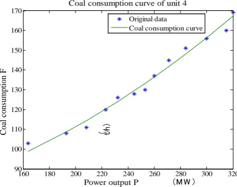
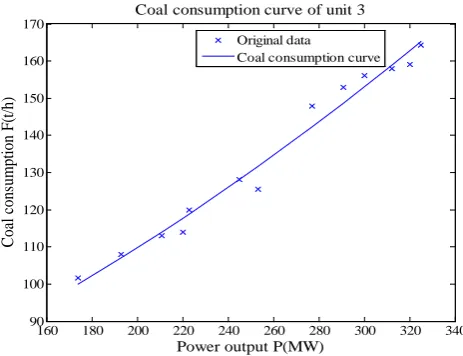
The same method can be used to fit coal consumption curve of the other three units, and the fitting results as shown in Figures 2-4.

Coal consumption curve equations of each unit are fitted by genetic algorithm, which are:

2

1 0.000285792906471322 1 0.152295463223784 1 49.7469230797674

F = P + P+

2

2 0.000471686919621979 2 0.175779299648337 2 43.0063408707241

(3)

[image:3.595.88.540.103.355.2]

Table 1. Power output-coal consumption table.

1# unit 2# unit 3# unit 4# unit

Power output (MW)

Coal consumption

(t/h)

Power output (MW)

coal consumption

(t/h)

Power output (MW)

coal consumption

(t/h)

Power output (MW)

coal consumption

(t/h)

189.85 90.00 170.00 85.00 174.00 101.62 163.70 103.00

217.59 95.00 190.00 93.00 192.92 107.96 192.96 108.00

220.00 96.00 205.92 100.00 210.83 113.02 208.15 111.00

240.00 104.00 220.00 107.00 220.00 114.00 222.96 120.00

250.00 105.00 230.00 112.00 222.92 120.00 232.22 126.00

260.00 111.00 240.00 107.00 245.00 128.14 244.81 128.00

271.86 112.00 250.00 117.00 253.39 125.46 252.96 130.00

280.00 116.00 260.00 123.00 277.08 147.91 260.00 137.00

290.00 114.00 277.00 128.00 290.83 153.02 271.10 145.00

300.00 123.00 296.00 131.00 300.00 156.05 284.07 151.00

310.00 122.00 300.00 137.00 312.08 158.00 300.00 156.00

315.00 126.00 318.00 148.00 320.00 159.00 315.00 160.00

[image:3.595.160.439.369.597.2]

320.00 130.00 320.00 150.00 325.00 164.31 320.00 169.20

Figure 1. Coal consumption curve of unit 1.

2

3 3

0.000502891284569065P +0.184153363892838P +52.6593691773213

2

4 0.00101282244303650 4 0.0599965442023200 4 83.1580882142092

F = P − P +

4. Coal Consumption Curve Fitting of the Thermal Power Based on Least Square

Method

For comparison purposes, methods and results of least squares fitting curve are given.

180 200 220 240 260 280 300 320

85 90 95 100 105 110 115 120 125 130

Power output P （M W ）

C

oa

l c

ons

um

pt

ion F

（ t/h）

Coal consumption curve of unit 1

Original data

(4)

[image:4.595.180.416.90.276.2] [image:4.595.180.413.307.485.2]

160 180 200 220 240 260 280 300 320

80 90 100 110 120 130 140 150

C

oa

l c

ons

um

pt

ion F

（ t/h）

Original data

Coal consumption curve

160 180 200 220 240 260 280 300 320 340

100 110 120 130 140 150 160 170

C

oa

l c

ons

um

pt

ion F

（ t/h）

Original data

160 180 200 220 240 260 280 300 320

90 100 110 120 130 140 150 160 170

C

oa

l c

ons

um

pt

ion F

（ t/h）

Original data

[image:4.595.181.413.519.702.2]

(5)

Set ϕ ϕ₀, ₁,...,ϕn are the functions of linear independence on C a b[ , ], and let Φ =span{ϕ ϕ0, 1,...,ϕn}. Set ( )

f x be a given discrete function on m+1 nodes which are a=x₀<x₁< <... xm=b, least squares method is

find s*∈ Φ to make * 2 2

0 0

( )[ ( ) ( )] min ( )[ ( ) ( )]

m m

j j j j j j

s

j j

x f x s x x f x s x

ρ ρ

∈Φ

= =

− = −

∑

, where ρ( )x is weight func-

tion on [ , ]a b . Then we call s x*( ) as the least squares solution for f x( ) which on m+1 nodes, also called as the least squares fitting [6].

According to above principle, the coal consumption curve which is used by quadratic polynomial is:

2

F =mP +tP+k (1) where

F—coal consumption of the unit power supply (t/h);

P—generation power of the unit (MW);

, ,

m t k—Energy consumption characteristic parameters.

Use least squares method to determine the binomial coefficient m t k, , . Set there are n experiments discrete data points (F_i, P_i)

Let 2 2

1

( )

n

i i i

i

J mP tP k F

=

∑

+ + − , to make the J minimum, and then let:

2 2

1

2 ( ) 0

n

i i i i

i J

P mP tP k F

m =

∂ ₌ ₊ _{+ −} ₌

∂

∑

(2)

2

1

2 ( ) 0

n

i i i i

i J

P mP tP k F

t =

∂

= + + − =

∂

∑

(3)

2

1

2( ) 0

n

i i i

i J

mP tP k F

k =

∂

= + + − =

∂

∑

(4)

After put in order we can get:

4 3 2 2

1 1 1 1

( ) ( ) ( ) ( )

n n n n

i i i i i

i i i i

P m P t P k F P

= = = =

+ + =

∑

(5)

3 2

1 1 1 1

( ) ( ) ( ) ( )

n n n n

i i i i i

i i i i

P m P t P k F P

= = = =

+ + =

∑

(6)

2

1 1 1

( ) ( )

n n n

i i i

P m P t nk F

= = =

+ + =

∑

(7)

Coal consumption parameters m t k, , can be obtained by solve the linear equations.

Using least square method to fit coal consumption curve, and the results as shown in Figures 5-8. Coal consumption curve equations of each unit are fitted by least square method, which are:

2

1 0.000580241018611 0.00488999810271 1 67.81118406745974

F = P + P+

2

2 0.0004332771431 2 0.19523379092699 2 40.62061826123973

F = P + P +

2

3 0.0004136575969 3 0.22857182978488 3 47.30730098461958

F = P + P +

2

4 0.00102118730423 4 0.06561283911416 4 84.01621840672190

F = P − P +

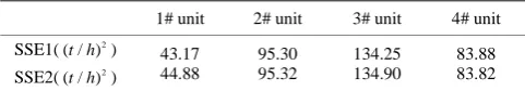
5. Fitting Error Analysis

The curve fitting is good or not judged by SSE (sum of square error), the sum of square error are obtained by these two algorithms as shown in Table 2.

Notes: SSE1 is sum of square error based on genetic algorithm and SSE2 is sum of square error based on least square method in the table.

(6)

[image:6.595.181.413.90.276.2] [image:6.595.180.415.308.492.2]

180 200 220 240 260 280 300 320

85 90 95 100 105 110 115 120 125 130

Power output P(MW)

C

oa

l c

ons

um

pt

ion F

(t

/h)

Original data

160 180 200 220 240 260 280 300 320

80 90 100 110 120 130 140 150

Power output P(MW)

C

oa

l c

ons

um

pt

ion F

(t

/h)

Original data

160 180 200 220 240 260 280 300 320 340 90

100 110 120 130 140 150 160 170

Power output P(MW)

C

oa

l c

ons

um

pt

ion F

(t

/h)

Original data

[image:6.595.181.413.524.702.2]

(7)

[image:7.595.181.415.87.270.2]

Table 2. Error sum of square.

1# unit 2# unit 3# unit 4# unit

SSE1( 2

( / )t h ) SSE2( 2

( / )t h )

43.17 44.88

95.30 95.32

134.25 134.90

83.88 83.82

genetic algorithm is significantly better than based on least square method, the original data are more fall on the curve or distributed around the curve, and more truly reflect the relationship between coal consumption and power output.

6. Conclusion

The experiments show that it is practicable use genetic algorithm to fit coal consumption curve. From the fitting results can be seen that the fitting curve can approximate the original data points, and it can better predict the coal consumption trend. But genetic algorithm also has its shortcomings, premature convergence, non direction-al genetic operator, and every time the search results are not fixed, these problems are expected next step to be improved.

References

[1] Wu, J., Ma, X. and Hou, R. (2011) Optimization of APF LCL Output Filter Based on Genetic Algorithm. Transactions of China Electrotechnical Society, 26, 159-164.

[2] Ma, X.-F. and Cui, H.-J. (2011) An Improved Genetic Algorithm for Distribution Network Planning With Distributed Generation. Transactions of China Electrotechnical Society, 26, 175-181.

[3] Wang, X.-P. (2002) Genetic Algorithms—Theory, Application and Software Implementation. Xi’an Jiaotong Univer-sity Press.

[4] Zhou, W.-Y., Lü, F.-P. and Li, H. (2013) Method for the Combination of Power System Operation Mode Based on Genetic Algorithm. Power System Protection and Control, 41, 51-55.

[5] Zhao, L.-Q. (2008) Research on the Plant’s Optimal Unit Commitment. North China Electric Power University. [6] Liu, X. (2007) Research on the Plant’s Optimal Load Dispatch and Unit Commitment of Thermal Power Plant Based

on Genetic Algorithm. North China Electric Power University.

160 180 200 220 240 260 280 300 320

100 110 120 130 140 150 160 170

Power output P(MW)

C

oa

l c

ons

um

pt

ion F

(t

/h)

[image:7.595.177.418.317.359.2]