Computational Studies on Detecting a Diffusing Target in a Square Region by a Stationary or Moving Searcher

American Journal of Operations Research, 2015, 5, 47-68

Published Online March 2015 in SciRes. http://www.scirp.org/journal/ajor http://dx.doi.org/10.4236/ajor.2015.52005

Computational Studies on Detecting a

Diffusing Target in a Square Region

by a Stationary or Moving Searcher

Hongyun Wang1, Hong Zhou2

1_{Department of Applied Mathematics and Statistics, Baskin School of Engineering, University of California,} Santa Cruz, USA

2_{Department of Applied Mathematics, Naval Postgraduate School, Monterey, USA} Email: [email protected], [email protected]

Received 6 February 2015; accepted 24 February 2015; published 28 February 2015

Copyright © 2015 by authors and Scientific Research Publishing Inc.

This work is licensed under the Creative Commons Attribution International License (CC BY).

http://creativecommons.org/licenses/by/4.0/

Abstract

In this paper, we compute the non-detection probability of a randomly moving target by a statio-nary or moving searcher in a square search region. We find that when the searcher is statiostatio-nary, the decay rate of the non-detection probability achieves the maximum value when the searcher is fixed at the center of the square search region; when both the searcher and the target diffuse with significant diffusion coefficients, the decay rate of the non-detection probability only depends on the sum of the diffusion coefficients of the target and searcher. When the searcher moves along prescribed deterministic tracks, our study shows that the fastest decay of the non-detection pro- bability is achieved when the searcher scans horizontally and vertically.

Keywords

Diffusing Target, Non-Detection Probability, Search Theory, Optimal Search Path

1. Introduction

Search problems arise commonly in many diverse areas [1]. For instance, we look for a missing key or person, the police officers search for fugitives, and prospectors explore for mineral deposits. Systematic research on search problems is now commonly known as search theory, which traces its root to the need of detecting sur-faced U-boats either visually from aircraft or with radar during World War II [2]-[7].

a moving target encountering a moving searcher. Much of the literature prior to the 1970s focuses on stationary targets. A comprehensive survey on research literature on moving targets has been provided by Benkoski et al.

[8].

In [9], Eagle considered the problem of a stationary searcher looking for a single moving target. He obtained an analytical expression for the non-detection probability of a randomly moving target encountering a stationary sensor when the search region was a disk and the cookie-cutter detector was fixed at the center of the search re-gion. Mangel [10] [11] looked at the problem where a target was assumed to move in the plane and the searcher in space. Optimal search path problems have been addressed by Washburn [12] [13], Eagle and his co-workers

[14]-[17]. The conflict between simplicity and optimality in searching for a 2-D stationary target was dealt with by Washburn [18]. A sequential approach to detect static targets with imperfect sensors such as tower-mounted cameras and satellites was presented by Wilson et al. [19]. Majumdar and Bray derived the survival probability of a tracer particle moving along a straight line in the presence of diffusing traps in the plane [20]. Fernando and Sritharan calculated the non-detection probability of infinitely many diffusing Brownian targets by a moving searcher which travels along a deterministic path with constant speed in the two-dimensional plane [21]. In this paper, we compute the non-detection probability of a diffusing Brownian target in the presence of a stationary or moving searcher in a square region. We study the effect of sweeping paths by considering five scenarios: the search may 1) diffuse randomly, 2) move along a circular or square loop, 3) move along a spiral, 4) move along a square spiral, and 5) scan horizontally and vertically.

2. Problem Setup

Consider a square region with half width RA, centered at the origin in the two-dimensional space. Mathemati-cally, the square can be described as

[

−R RA, A

] [

× −R RA, A

]

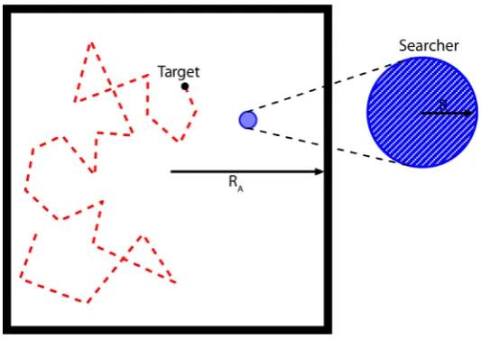
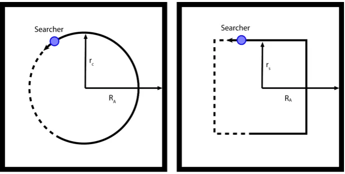
. In our search problem, this square is the search re-gion in which the target undergoes Brownian diffusion.

[image:2.595.180.447.472.660.2]

Suppose the searcher is capable of detecting a target instantly when the target gets within distance R to the location of the searcher and there is no possiblity of detection when the target range is greater than R. That is, the searcher covers a disk of radius R centered at the location of the searcher. The expression “cookie-cutter de-tection rule” is often used to describe this type of sensor modeling. One major criticisim of the cookie-cutter rule is based on the argument that fluctuations in the performance of detection equipment and human operators make it extremely rare to have a critical detection range R. Despite the limitations, the cookie-cutter model offers the simplest and most practical method to model sensors including radar, eyeball, infra-red, and low level TV. We illustrate the search problem in Figure 1.

Figure 1. A schematic illustration of a diffusing target in a square search region of half width RA in the presence of a searcher. The searcher may be fixed, may

undergo Brownian diffusion, or may be moving with velocity vs along a

H. Wang, H. Zhou

We carry out Monte Carlo simulations to study the time evolution of the non-detection probability, respec-tively, when the searcher is fixed at various locations, when the searcher undergoes Brownian diffusion with various values of diffusion coefficient, and when the searcher is moving along various prescribed deterministic paths.

Let Dt denote the diffusion coefficient of the target, and Ds the diffusion coefficient of the searcher. In our simulations, we choose the parameters as follows:

75 2 100 A s t R R D D = = + = (1)

and consider five problems below.

3. Problem 1: Diffusing Target and Diffusing Searcher

We look at the situation where the target and the searcher are diffusing with various diffusion coefficients. The case of a stationary searcher is the special case with Ds=0.

In our numerical discretization,

( ) ( )

(

)

( ) ( )

(

)

, is the location of the target at time

, is the location of the searcher at time .

j

t t j

s s j

t j t

x j y j t

x j y j t

= ∆

In Monte Carlo simulations, we advance the target and the searcher in time according to

( )

₍

₎

( )

₍

₎

(

)

(

( ) ( )

)

(

)

( )

₍

₎

( )

₍

₎

(

)

(

( ) ( )

)

(

)

1 2 3 4

1 , 1 , 2 ,

1 , 1 , 2 ,

tem tem

t t t t t

tem tem

s s s s s

x j y j x j y j D t W W

x j y j x j y j D t W W

+ + = + ∆

+ + = + ∆ (2)

where W1, W2, W3, and W4 are independent samples of standard normal distribution (mean 0, variance 1).

To enforce the reflection condition at the boundary of the square search region, we calculate the new positions of target and searcher as

(

)

(

( )

₍

₎

)

(

)

(

( )

₍

₎

)

(

)

(

( )

₍

₎

)

(

)

(

( )

₍

₎

)

1 Reflection 1

1 Reflection 1

1 Reflection 1

1 Reflection 1

tem

t A t A

tem

t A t A

tem

s A s A

tem

s A s A

x j R x j R

y j R y j R

x j R x j R

y j R y j R

+ = ⋅ +

+ = ⋅ +

+ = ⋅ +

+ = ⋅ +

(3)

where function Reflection

( )

x is defined as

( )

(

)

Reflection x ≡ − −1 2 mod x+1, 4 .

It is straightforward to verify that

( )

( )

( )

Reflection , 1 1

Reflection 2 , 1 3

Reflection 2 , 3 1.

x x x

x x x

x x x

= − ≤ ≤

= − < < = − − − < < −

(4)

The target is labeled as “detected” at tj if the distance between the target and the searcher is less than the detection range R:

( )

( )

(

)

2

(

( )

( )

)

2

.

t s t s

Once the target is detected, that particular Monte Carlo run is terminated and another independent Monte Carlo run is started. To speed up the simulation, multiple Monte Carlo runs are carried out in parallel.

Let

(

x y0, 0

)

be the initial location of the searcher. In Monte Carlo simulations, the initial location of the

target is selected randomly and uniformly from the part of the square search region that is outside the disk of ra-dius R centered at

(

x y0, 0

)

(i.e., outside the the searcher’s detection area at t=0).

For each set of parameter values, we repeat the Monte Carlo run N=100000 times. The non-detection pro- bability is calculated by averaging over 100,000 repeats.

In Problem 1, we select the time step ∆t1 such that

(

)

1

1

2 .

8 s t

D +D ∆ =t R (6)

That is, the root-mean-square of the displacement between the target and the searcher in time period ∆t1 is

no more than one eighth of the detection radius of the searcher.

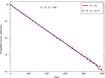
We first examine the accuracy of our Monte Carlo simulations in the case of

(

x y0, 0

) ( )

= 0, 0 , Dt =100, Ds =0.

Figure 2 compares the non-detection probabilities obtained with two different time steps: ∆ = ∆t t1 as given

in (6) and ∆ = ∆t t1 4. Figure 2 demonstrates that the time step ∆t1 is small enough. In Problem 1, we use 1

t

∆ as the time step unless specified otherwise.

Figure 3 compares the non-detection probabilities obtained in 7 independent Monte Carlo simulations, each

simulation consisting of N=100000 repeats. The parameter set is the same as in Figure 2. From Figure 3, we can see that the number of repeats, N=100000, is large enough.

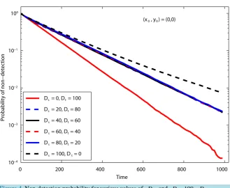
[image:4.595.145.484.430.684.2]

Next, we explore several cases that satisfy Ds+Dt =100 ranging from Ds =0 to Ds=100. When Ds =0, the searcher is fixed; when Ds =100, we have Dt= 0 and the target is fixed. The initial location of the searcher is

(

x y0, 0

) ( )

= 0, 0 .

Figure 4 plots the non-detection probability for various values of Ds and Dt =100−Ds. The fastest decay

of the non-detection probability occurs when Ds=0 (i.e., when the searcher is fixed at

( )

0, 0 ). The decay of

[image:5.595.145.495.79.335.2]

H. Wang, H. Zhou

[image:5.595.149.479.368.638.2]

Figure 3. Comparison of results from 7 independent Monte Carlo simulations. Each simu- lation consists of N=100000 repeats.

Figure 4.Non-detection probability for various values of Ds and Dt=100−Ds.

the non-detection probability is slowed down when the searcher diffuses with Ds>0. This observation indi-cates that the best location for the searcher is at the center

( )

0, 0 ; diffusion with Ds>0 randomizes the searcher location and decreases the decay rate of the non-detection probability. Notice that in Figure 4 when

0 s

D > , the decay rate of the non-detection probability is no longer sensitive to changes in Ds as along as

s t

detection probability is affected only by the relative diffusion

(

Ds+Dt

)

between the searcher and the target. Finally, in Figure 4, the slowest decay of the non-detection probability occurs when Dt =0. Recall that the ini-tial location of the target is randomized and is most likely away from the center. Dt =0 fixes the target at its initial off-center location and makes it less likely for the diffusing searcher to encounter the target. In the case of

0 t

D = , if we switch the roles of the target and the searcher, we see that when a searcher is fixed at an off-center location with no diffusion, the non-detection probability decays the slowest. Thus, for a given relative diffusion between the searcher and the target

(

Ds+Dt

)

, Figure 4 suggests the following observations:

1) the decay rate of the non-detection probability is the largest when the searcher is fixed at the center; 2) when both the searcher and the target are diffusing with significant diffusion coefficients, the decay rate of the non-detection probability is lower and is independent of Ds as long as Ds+Dt is a fixed constant;

3) when the searcher is fixed at a location significantly off center, the decay rate of the non-detection proba-bility is even lower.

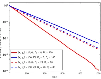
To further test these observations, we compare the decay rates of the non-detection probability for 4 sets of parameters

(

) ( )

( )

(

)

(

) ( )

(

)

(

) (

)

(

)

(

)

0 0 0 0 0 0 0 0

Set 1: , 0, 0 , 0

the searcher is fixed at 0, 0

Set 2 : , 0, 0 , 20

both the searcher and the target have significant diffusion

Set 3 : , 50, 50 , 20

both the searcher and the target have significant diffusion

Set 4 : , 50,

s

s

s

x y D

x y D

x y D

x y = = = = = = =

(

)

(

)

(

)

50 , 0

the searcher is fixed at 50, 50 . s

D =

Based on the observations 1)-3) above, we expect that set 1 produces the fastest decay of the non-detection probability; sets 2 and 3 yield similar decay rates, lower than that of set 1; and set 4 gives the slowest decay rate of the non-detection probabilty.

Figure 5 compares the results for these four parameter sets. The results in Figure 5 confirm what we

pre-dicted based on observations 1)-3). Hence, these results provide further support for observations 1)-3). Figure 5

also indicates that when the searcher has significant diffusion, its inital location does not matter.

Next we study the case of a fixed searcher

(

Ds =0

)

. We investigate how the searcher’s location affects the decay rate of the non-detection probability. Figure 6 shows that for a stationary searcher, the decay rate of the non-detection probability decreases as the distance between the searcher and the center is increased.

In summary, for Problem 1, we conclude that a) when both the searcher and the target have significant diffu-sion, the decay rate of non-detection probability is independent of the initial location and is independent of Ds as long as Ds+Dt is fixed; b) for a given value of Ds+Dt, the fastest decay of non-detection probability oc-curs when the searcher is fixed at the center

( )

0, 0 .

Next, we study the case where the searcher moves with a constant velocity vs along a prescribed determinis-tic loop.

4. Problem 2: Searcher Moving along a Loop

We consider the situation where the target diffuses with diffusion coefficient Dt =100 and the searcher moves with velocity vs along a loop (a circular or a square loop). We select velocity vs as follows.

Let τ1 be the time scale of the target diffusing a root-mean-square distance of 2R along a given direction.

Time scale τ1 can be viewed as the time scale of the target probability distribution relaxing to erase the mark

swept by the searcher. Time scale τ1 is given by

( )

2 1

2D_tτ = 2R . (7)

[image:7.595.151.481.81.339.2]

H. Wang, H. Zhou

Figure 5. Comparison of decay rates of non-detection probability for 4 sets of parameter values.

Figure 6. The effect of the searcher location on the decay rate of non-detection probability when the searcher is fixed

(

Ds=0

)

.

where the target velocity is neither too small nor too large. Specifically, we consider the case where the distance traveled by the searcher in time τ1 is a small multiple of 2R:

( )

1 2 .

s

[image:7.595.149.481.374.630.2]

We pick α=10. The corresponding velocity is found to be

( )

( )

2

(

)

2

500.

2 2

t s

t

R D

v

R

R D

α

α

= = = (9)

In all the simulations below, we use vs =500.

In Problem 2, for each set of parameter values, we repeat the Monte Carlo run N=200000 times. We also use a smaller time step (see below). The increased time and ensemble resolution is made possible by the fact that when the searcher moves along a loop, the non-detection probability decays faster than in the optimal case of Problem 1 where the searcher is fixed at the center. With fast decay of the non-detection probability, detections occur early and consequently Monte Carlo runs on average end early in simulations.

We select the time step ∆t2 such that

2 2

1

2 .

12

t s

D t∆ + ∆ ≤v t R (10)

That is, the root-mean-square diffusion of the target toward the searcher in time ∆t2 plus the distance

tra-veled by the searcher in time ∆t2 does not exceed one twelfth of the detection radius of the searcher.

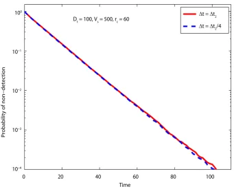
We first examine the accuracy of our Monte Carlo simulations when the searcher moves along a circle of ra-dius rc=60 with velocity vs =500, as illustrated in the left panel ofFigure 7.

Figure 8 compares the non-detection probabilities obtained with two time steps: ∆ = ∆t t2 given in (10) and

2 4

t t

∆ = ∆ . Figure 8 tells us that the time step ∆t2 is small enough. In Problem 2, we use ∆t2 as the time

step unless specified otherwise.

Figure 9 compares the non-detection probabilities obtained from 7 independent Monte Carlo simulations,

[image:8.595.141.487.492.667.2]

each consisting of N=200000 repeats. Figure 9 demonstrates that N=200000 is adequate for accurately capturing the decay of the non-detection probability.

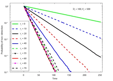
Figure 10 shows the effect of the circle radius rc on the time evolutions of the non-detection probability.

When the searcher moves along a small circle (small rc), the non-detection probability decays moderately fast-er than in the case of the searchfast-er being fixed at the centfast-er

(

rc=0

)

. When we expand the circle path from

10 c

r = to rc =20, to rc=40,, the decay rate of the non-detection probability increases. The optimal ra-dius for the fastest decay of the non-detection probability is about rc(optimal) =60. When the circle path is ex-panded beyond rc =60, the decay rate of the non-detection probability is reduced slightly from the optimal value. When rc is large and the circle path is close to the boundary of the square search region, it takes long time for a target initially near the center to diffuse the long distance to encounter the searcher. Likewise, when

Figure 7. The searcher moves along a prescribed loop with velocity vs. (a) The prescribed

loop is a circle of radius rc; (b) The prescribed loop is a square of half width rs. (a) The

searcher moves along a circle with velocity vs; (b) The searcher moves along a square with

[image:9.595.144.486.83.358.2]

H. Wang, H. Zhou

Figure 8. Comparison of numerical results obtained, respectively, with time step ∆ = ∆t t2 and refined time step ∆ = ∆t t2 4, for the case of searcher moving along a circle of radius

60

c

r = with velocity vs=500. Time step ∆t2 is described in the text.

[image:9.595.141.487.384.692.2]

Figure 10.Results for the case of the searcher moving along a circle of radius rc. Shown

here are time evolutions of non-detection probability for various values of circle radius rc.

c

r is small and the circle path covers just the area near the center, it takes long time for a target initially near the boundary to diffuse the long distance to encounter the searcher. Thus, the optimal circle path is the one that is the best compromise for taking care both the area around the center and the area near the boundary of the search region. Intuitively, one may conjecture that the optimal circle path is the one that divides the whole search re-gion into 2 equal parts:

area inside the optimal circle=area outside the optimal circle.

The optimal circle radius based on the intuitive conjecture above is

(optimal)

(

2

)

2 2

59.84. π

A c

R

r = = (11)

The results of Monte Carlo simulations in Figure 10 strongly support this conjecture.

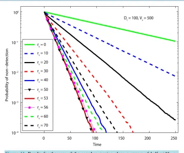
Next we study the case of the searcher moving along a square path of half width rs with velocity vs =500, as illustrated in the right panel of Figure 7.

Figure 11 shows the effect of half width rs on the time evolutions of the non-detection probability. When

the searcher moves along a small square path (small rs), the non-detection probability decays moderately faster than in the case of the searcher being fixed at the center

(

rs=0

)

. When we expand the square path from

10 s

r = to rs =20, to rs=40,, the decay rate of the non-detection probability increases. The optimal half width for fastest decay of the non-detection probability is about (optimal)

= 53

s

[image:10.595.141.518.79.350.2]

[image:11.595.134.494.77.375.2]

H. Wang, H. Zhou

Figure 11. Results for the case of the searcher moving along a square of half width r_s. Shown here are time evolutions of non-detection probability for various values of half width

s r.

( )

(

)

2

optimal 2 2

53.03. 2

A c

R

r = = (12)

The results of Monte Carlo simulations inFigure 11 strongly support this conjecture.

Before we end this section, we calculate and compare the decay rates of the non-detection probability for the three optimal cases we have considered so far. The decay rate of the non-detection probability, denoted by

decay

k , is calculated by fitting a straight line to data points of time vs log(non-detction probability).

1) For the case of diffusing target and diffusing searcher with fixed total diffusion Ds+Dt =100, the optimal (the fastest) decay rate of the non-detection probability is achieved when the searcher is fixed at the center. The optimal decay rate is found to be

(

)

2

decay searcher fixed at the center 0.895 10 .

k = × −

2) For the case of the searcher moving along a circle of radius rc with velocity vs =500, the optimal (the fastest) decay rate of the non-detection probability is achieved when rc=60. The optimal decay rate is

(

)

2

decay sweeping circle of radius c 60 9.21 10 .

k r = = × −

3) For the case of the searcher moving along a square of half width rs with velocity vs =500, the optimal (the fastest) decay rate of the non-detection probability is achieved when rs =53. The optimal decay rate is

(

)

2

decay sweeping square of half width s 53 9.88 10 .

k r = = × −

Out of these 3 cases, square loop of half width rs=53 yields the fastest decay of the non-detection

probabil-ity with decay rate 2

decay 9.88 10

k = × − .

5. Problem 3: Searcher Moving along a Spiral

We consider the situation where the target diffuses with diffusion coefficient Dt =100 and the searcher moves along a path consisting of rotated spiral loops, which we will describe in detail below. In all simulations of the searcher sweeping a prescribed path, we use velocity vs =500. The selection of vs =500 has been discussed in Problem 2. In Problem 3, we select numerical parameters as follows: each Monte Carlo simulation is repeated

800000

N= times and the time step ∆t3 satisfies

3 3

1

2 .

12

t s

D t∆ + ∆ ≤v t R (13)

The increase in number of repeats from N=200000 to N=800000 is made possible by that the detection is faster in Problem 3, and as a result, the Monte Carlo simulations, on average, end earlier than in Problems 1 and 2.

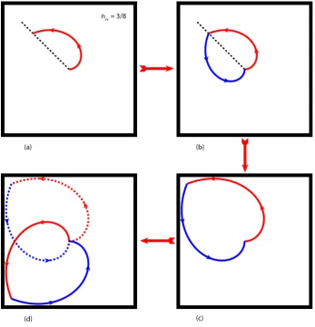
[image:12.595.140.488.273.635.2]

A spiral path is a sequence of rotated spiral loops and is specified by the number of revolutions nrv in each spiral. The construction of a spiral path with nrv =3 8 is shown in Figure 12. Each spiral loop in the spiral

Figure 12.A spiral path is a sequence of rotated spiral loops and is specified by the number of revolutions n_rv in each forward spiral. A spiral path is constructed in 4 steps. (a) A spiral of

rv

H. Wang, H. Zhou

path is formed by a forward spiral starting at the origin and a backward spiral back to the origin. We use the Archimedean spiral. The forward spiral of nrv revolutions can be mathematically described as

(

0

)

0

( )

Forward spiral : r= ⋅ −b θ θ , 0≤ −θ θ ≤nrv 2π .

We select the starting angle θ0 such that the ending angle θ0+nrv

( )

2π is at a diagonal, pointing to a cor-ner of the square search region (Figure 12(a)). For nrv =3 8, we select θ =0 0; for nrv=1, we select θ =0 π 4.

The backward spiral is the mirror reflection image of the forward spiral with respect to the line of ending angle

(Figure 12(b)). Mathematically the backward spiral is

( ) (

)

(

0

)

( )

0

( )

Backward spiral : r= ⋅b 2nrv 2π − θ θ− , nrv 2π ≤ −θ θ ≤2nrv 2π .

Recall that in our problem, the searcher moves along a path with a constant velocity. To use the spiral loop as the searcher’s sweeping path in simulations, we need to express

( )

θ,r as a function of arclength s. The ar-clength along the forward spiral is given by

( )

(

0

)

s θ = ⋅b g θ θ− (14)

where function g

( )

θ is the arclength in the special case of b=1 and θ =0 0:

( )

1

(

2

(

2

)

)

1 log 1 .

2

g θ = θ +θ + θ+ +θ (15)

Let sh be the arclength of the forward spiral (half the arclength of the spiral loop). Mathematically, it fol-lows that

( )

(

2π .

)

h rv

s = ⋅b g n (16)

For the forward spiral, 0≤ ≤s sh. The polar coordinates

( )

θ,r of the forward spiral are expressed as func-tions of arclength s using the inverse function of g

( )

θ .

( )

( )

1 0 1 , 0 , 0 h h s

s g s s

b

s

r s b g s s

b

θ θ −

−   = + _{ } ≤ ≤     = ⋅ _{ } ≤ ≤   (17)

For the backward spiral, sh≤ ≤s 2sh. The polar coordinates

( )

θ,r of the backward spiral are expressed as functions of arclength s as

( )

( )

( )

1 0 1 2

2 2π , 2

2

, 2 .

h

rv h h

h

h h

s s

s n g s s s

b

s s

r s b g s s s

b

θ θ −

− −   = + − _{ } ≤ ≤   −   = ⋅ _{ } ≤ ≤   (18)

In our numerical simulations, the inverse function 1

( )

g− ⋅ is evaluated by solving for θ in equation g

( )

θ =s

using Newton’s method.

The Cartesian coordinates of the spiral loop as functions of arclength s are written out based on the polar coordinates:

( ) ( )

(

( )

)

( ) ( )

(

( )

)

cos

sin . x s r s s

y s r s s θ θ

=

= (19)

( ) (

)

( )

(

)

( ) (

)

( )

(

)

0 2

0 2

0 2

0 2

max

min

max

min .

h

h

h

h

A s s

A s s

A s s

A s s

x s R R

x s R R

y s R R

y s R R

≤ ≤

≤ ≤

≤ ≤

≤ ≤

≤ −

≥ − −

≤ −

≥ − −

(20)

When sweeping the spiral loop, the Cartesian coordinates of the searcher as functions of time t are given by

( )

(

( )

)

( )

(

( )

)

cos

sin .

s s

s s

x r v t v t

y r v t v t θ θ

=

= (21)

This is the formula we use to update the searcher location in simulations.

[image:14.595.141.487.319.697.2]

After finishing sweeping one spiral loop, the searcher rotates the spiral loop by π 2 and starts sweeping along the rotated spiral loop (Figure 12(d)). This process is repeated until the target is detected.

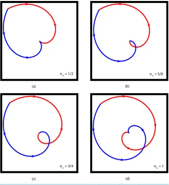
Figure 13 demonstrates four spiral loops, respectively, of nrv =1 2, of nrv =5 8, of nrv=3 4, and of

1 rv

n = . In each spiral loop, the forward spiral is shown in red and the backward spiral in blue. The correspond-ing spiral sweepcorrespond-ing path for the searcher contains a sequence of rotations of the spiral loop.

Figure 13. Four spiral loops corresponding to nrv=1 2, nrv=5 8, nrv=3 4, and nrv=1.

H. Wang, H. Zhou

Figure 14 depicts the time evolutions of the non-detection probability when the searcher sweeps various

spir-al paths. A spirspir-al path is specified by nrv, the number of revolutions in the forward spiral. Figure 14 compares the results for 9 values of nrv, ranging from nrv =1 8 to nrv =20. The fastest decay of the non-detection proba-bility occurs at n_rv(optimal) =5 8. The decay rates are almost the same among nrv =1 2, nrv =5 8, and nrv =3 4. The spiral loop of nrv =5 8 is shown in Figure 13(b). The corresponding spiral sweeping path is a sequence of ratations of the spiral loop. The decay rate of the non-detection probability at nrv =5 8 is

(

)

2

decay sweeping spiral path of rv 5 8 12.21 10 .

k n = = × −

We point out that the optimal decay rate given above for Problem 3 is faster (larger) than those of Problems 1 and 2.

6. Problem 4: Searcher Moving along a Square Spiral

Now we consider the situation where the target diffuses with diffusion coefficient Dt =100 and the searcher moves along a path consisting of rotated square spiral loops, which we will describe in detail below. The searcher moves with velocity vs =500, the same velocity as we used in Problems 2 and 3.

In Problem 4, we use the same numerical parameters as in Problem 3: each Monte Carlo simulation is re-peated N=800000 times and the time step ∆t4 satisfies

4 4

1

2 .

12

t s

D t∆ + ∆ ≤v t R (22)

A square spiral path is a sequence of rotated square spiral loops and is specified by the number of square lay-ers nsq in each forward square spiral. A square spiral loop is formed by a forward square spiral starting at the origin and a backward square spiral back to the origin.

[image:15.595.142.485.400.670.2]

We first focus on square spirals with unit inter-layer distance. A forward square spiral of nsq square layers is

Figure 14.Results for the case of searcher moving along various spiral paths. A spiral path is a sequence of ratations of a spiral loop and is specified by nrv, the number of revolutions in

described as follows. We cycle through 4 directions: positive x, positive y, negative x, negative y. If we start at

( )

0, 0 and sequentially go in each of 4 directions by a distance of 1, we obtain a unit square with its lower left corner at

( )

0, 0 . Mathematically, the construction of this unit square is concisely and conveniently denoted by

{

}

A unit square= 1,1,1,1 .

With this simple notation, the forward square spiral of nsq layers is described by

(

) (

)

{

}

Forward square spiral of n_sqlayers= 1,1, 2, 2, 3, 3,, 2n_sq−1 , 2n_sq−1 , 2n_sq, 2n_sq .

In this unit forard square spiral, the inter-layer distance is 1. Next we scale the unit forward square spiral to fit it to the search region. Let d be the inter-layer distance after the scaling. We select the inter-layer distance d as

1 4 A

sq

R d

n

= +

where RA is the half width of the search region. All square spirals in Problem 4 are scaled using the inter-layer distance d given above. The forward square spiral of 2 layers

(

n_sq =2

)

is shown in Figure 15(a).

We could select the backward square spiral as the mirror image of the forward square spiral with respect to

Figure 15. Forward square spirals and square spiral loops. (a) The forward square spiral of 2

sq

n = (2 layers); (b) The square spiral loop of n_sq=2, formed by concatenating the

for-ward and the backfor-ward square spirals; (c) The forfor-ward square spiral of nsq=3 (3 layers); (d)

[image:16.595.138.488.313.660.2]

H. Wang, H. Zhou

the line of angle 1 π

4 . If we do that, however, the backward square spiral will coincide with the forward square spiral in a substantial fraction of the path. Intuitively, that is not an efficient way of sweeping. We want the backward square spiral to cover the area between the layers of the forward square spiral so that together the forward and the backward square spirals have a better and more uniform coverage of the search region. We de-sign the backward square spiral to go between the layers of the forward square spiral. Mathematically, the backward square spiral is described by

(

) (

) (

) (

)

Backward square spiral of layers

1 1 1 1

2 , 2 , 2 1 , 2 1 , 2 2 , 2 2 , , 2, 2,1,1, , .

2 2 2 2

sq

sq sq sq sq sq sq

n

n n n n n n

 

=_ − − − − − − _

  

As in the situation for the forward square spiral, the backward square spiral is also scaled by the inter-layer distance d given above to fit it to the search region. The backward square spiral of 2 layers

(

nsq =2

)

is shown

in Figure 15(b) (blue line with filled circles). The square spiral loop is formed by combining the forward and

the backward square spirals. The square spiral loop of n_sq=2 is shown in Figure 15(b). The square spiral loop starts at the origin and returns to the origin at the end.

After finishing sweeping the square spiral loop, the searcher rotates the whole square spiral loop by π 2 and starts sweeping along the rotated square spiral loop. This process is repeated until the target is detected.

Figure 16 plots the time evolutions of the non-detection probability when the searcher sweeps various square

spiral paths. A square spiral path is specified by nsq, the number of square layers in the forward square spiral (see Figure 15). Figure 16 compares the results for 9 values of nsq, ranging from nsq=1 (the lowest possible value for nsq) to nsq =22. The fastest decay of the non-detection probability occurs at

(optimal) 3 sq

n = . The decay

rates are almost the same among n_sq =2, n_sq =3, and n_sq =4. The square spiral loop of n_sq =3 is shown in

Figure 15(d). The corresponding square spiral path is a sequence of ratations of the square spiral loop. The decay

Figure 16. Results for the case of the searcher moving along various square spiral paths. A square spiral path is a sequence of rotations of a square spiral loop and is specified by nsq,

[image:17.595.144.485.403.662.2]

rate of the non-detection probability at n_sq =3 is

(

)

2

decay sweeping square spiral path of sq 3 12.96 10 .

k n = = × −

We point out that the optimal decay rate given above for Problem 4 is faster (larger) than those of Problems 1, 2 and 3.

7. Problem 5: Searcher Scanning Horizontally and Vertically

Finally we consider the situation where the target diffuses with diffusion coefficient Dt =100, and the searcher scans horizontally and vertically back and forth. The detailed construction of the scan path will be described be-low. The searcher moves with velocity vs =500, the same velocity as we used in Problems 2, 3 and 4.

In Problem 5, we use the same numerical parameters as in Problems 3 and 4: each Monte Carlo simulation is repeated N=800000 times and the time step ∆t5 satisfies

5 5

1

2 .

12

t s

D t∆ + ∆ ≤v t R (23)

The scan path consists of forward horizontal scan, backward horizontal scan, forward vertical scan and back-ward vertical scan. A forback-ward horizontal scan is shown in Figure 17.

A forward horizontal scan is specified by 3 parameters: b the length of each horizontal scan line, d the inter scan line distance, and nsc the number of horizontal scan lines. Parameters b and d are shown in Figure 17. The distance from the first horizontal scan line to the last horizontal scan line is

(

n_sc−1

)

d. Since the searcher is scanning a square region, we set

(

sc 1

)

.

b= n − d

For each forward horizontal scan, there is an associated backward horizontal scan. The backward scan travels between the horizontal scan lines of the forward scan. The forward horizontal scan is mathematically described by

(

) ( )

(

) (

)

(

)

(

( )

1

)

Forward scan line 1: , , 0

Forward scan line : , 0, ,

, 1 j , 0 , 2, , _sc. x y b

j x y d

x y b − j n

∆ ∆ = ∆ ∆ =

∆ ∆ = − = 

[image:18.595.207.417.496.684.2]

The associated backward horizontal scan is mathematically described by

Figure 17.A forward horizontal scan and associated parameters. b

H. Wang, H. Zhou

(

) (

)

(

)

(

( )

)

Backward scan line 1: , 0, 2 ,

, 1nsc, 0

x y d

x y b

∆ ∆ = −

∆ ∆ = −

(

) (

)

(

)

(

( )

1

)

Backward scan line : , 0, ,

, 1 nsc j , 0 , 2, , 1

sc

j x y d

x y b − + j n

∆ ∆ = −

∆ ∆ = − =  −

(

) (

)

(

) (

)

Backward scan line : , 0, 2 ,

, , 0 .

sc

n x y d

x y b

∆ ∆ = −

∆ ∆ = −

The forward horizontal scan and the associated backward horizontal scan for nsc =5 are shown in Figure

18(a), Figure 18(b).

The vertical scans are exactly the same as the horizontal scans except that the roles of x and y are swapped. The forward vertical scan is

(

) ( )

(

) ( )

(

)

(

( )

1

)

Forward scan line 1: , 0,

Forward scan line : , , 0 ,

, 0, 1 j , 2, , _sc.

x y b

j x y d

x y b − j n

∆ ∆ = ∆ ∆ =

∆ ∆ = − = 

[image:19.595.137.488.349.687.2]

The associated backward vertical scan is

(

) (

)

(

)

(

( )

)

Backward scan line 1: , 2 , 0 ,

, 0, 1nsc

x y d

x y b

∆ ∆ = −

∆ ∆ = −

(

) (

)

(

)

(

( )

1

)

Backward scan line : , , 0 ,

, 0, 1nsc j , 2, , 1

sc

j x y d

x y b − + j n

∆ ∆ = −

∆ ∆ = − =  −

(

) (

)

(

) (

)

Backward scan line : , 2 , 0 ,

, 0, .

sc

n x y d

x y b

∆ ∆ = −

∆ ∆ = −

The forward vertical scan and the associated backward vertical scan for nsc=5 are shown in Figure 18(c),

Figure 18(d).

To scan the square search region of half width RA, we set

(

)

2

, 1 .

1 2 A

sc sc

R

d b n d

n

= = −

−

Thus, for a square of given half width RA, a scan path is completely specified by nsc, the number of scan lines in each scan.

[image:20.595.143.487.412.670.2]

The searcher sequentially cycles through forward horizontal scan, backward horizontal scan, forward vertical scan and backward vertical scan. This process is repeated until the target is detected.

Figure 19 shows the time evolutions of the non-detection probability when the searcher scans horizontally

and vertically. A scan path is specified by nsc, the number of scan lines in each forward scan. Figure 19 com-pares the results for 9 values of nsc, ranging from nsc=2 (the lowest possible value for nsc) to nsc=30. The fastest decay of the non-detection probability occurs at n(_scoptimal)=11. The decay rates are almost the same among nsc=10, nsc=11, and nsc =12. The decay rate of the non-detection probability at nsc=11 is

Figure 19. Results for the case of searcher scanning horizontally and vertically. The horizon-tal and vertical scan paths are shown in Figure 18. A scan path is specified by nsc, the

H. Wang, H. Zhou

(

)

2

decay sweeping scan path of sc 11 13.58 10 .

k n = = × −

We point out that the optimal decay rate given above for Problem 5 is faster (larger) than those of Problems 1, 2, 3 and 4.

8. Summary

This paper calculated the non-detection probability of a diffusing target in the presence of a stationary or moving searcher. It is found that when the searcher is fixed, the decay rate of the non-detection probability attains the maximum value when the search is fixed at the center of the square search region. When both the searcher and the target diffuse with significant diffusion coefficients, the decay rate of the non-detection probability only de-pends on the sum of the diffusion coefficients of the target and searcher. When the searcher moves along various deterministic trajectories, the fastest decay of the non-detection probability is obtained when the searcher scans horizontally and vertically.

Acknowledgements and Disclaimer

Hong Zhou would like to thank Professor James Eagle, Professor Sivaguru Sritharan and Professor Jim Scrofani for stimulating discussions. The views expressed in this document are those of the authors and do not reflect the official policy or position of the Department of Defense or the US Government.

References

[1] Koopman, B.O. (1999) Search and Screening: General Principles with Historical Applications. The Military Opera-tions Research Society, Inc., Alexandria.

[2] Chudnovsky, D.V. and Chudnovsky, G.V. (1989) Search Theory: Some Recent Developments. Marcel Dekker, Inc., New York.

[3] Chung, T.H., Hollinger, G.A. and Isler, V. (2011) Search and Pursuit-Evasion in Mobile Robotics: A Survey. Auto-nomous Robots, 31, 299-316. http://dx.doi.org/10.1007/s10514-011-9241-4

[4] Dobbie, J.M. (1968) A Survey of Search Theory. Operations Research, 16, 525-537.

http://dx.doi.org/10.1287/opre.16.3.525

[5] Stone, L.D. (1989) Theory of Optimal Search. 2nd Edition, Academic Press, San Diego.

[6] Stone, L.D. (1989) What’s Happened in Search Theory Since the 1975 Lanchester Prize? Operations Research, 37, 501-506. http://dx.doi.org/10.1287/opre.37.3.501

[7] Washburn, A.R. (2002) Search and Detection. Topic in Operation Research Series. 4th Edition, INFORMS, Catons-ville.

[8] Benkoski, S.J., Monticino, M.G. and Weisinger, J.R. (1991) A Survey of the Search Theory Literature. Naval Research Logistics, 38, 469-494. http://dx.doi.org/10.1002/1520-6750(199108)38:4<469::AID-NAV3220380404>3.0.CO;2-E

[9] Eagle, J.N. (1987) Estimating the Probability of a Diffusing Target Encountering a Stationary Sensor. Naval Research Logistics, 34, 43-51. http://dx.doi.org/10.1002/1520-6750(198702)34:1<43::AID-NAV3220340105>3.0.CO;2-6

[10] Mangel, M. (1981) Search for a Randomly Moving Object. SIAM Journal on Applied Mathematics, 40, 327-338.

http://dx.doi.org/10.1137/0140028

[11] Mangel, M. (1981) Optimal Search for and Mining of Underwater Mineral Resources. SIAM Journal on Applied

Ma-thematics, 43, 99-106. http://dx.doi.org/10.1137/0143008

[12] Washburn, A.R. (1995) Dynamic Programming and the Backpacker’s Linear Search Problem. Journal of

Computa-tional and Applied Mathematics, 60, 357-365. http://dx.doi.org/10.1016/0377-0427(94)00038-3

[13] Washburn, A.R. (1998) Branch and Bound Methods for a Search Problem. Naval Research Logistics, 45, 243-257.

http://dx.doi.org/10.1002/(SICI)1520-6750(199804)45:3<243::AID-NAV1>3.0.CO;2-7

[14] Dell, R.F., Eagle, J.N., Martins, G.H.A. and Santos, A.G. (1996) Using Multiple-Searchers in Constrained-Path, Mov-ing-Target Search Problems. Naval Research Logistics, 43, 463-480.

http://dx.doi.org/10.1002/(SICI)1520-6750(199606)43:4<463::AID-NAV1>3.0.CO;2-5

[15] Eagle, J.N. (1984) The Optimal Search for a Moving Target When the Search Path Is Constrained. Operations Re-search, 32, 1107-1115. http://dx.doi.org/10.1287/opre.32.5.1107

Search Problem. Operations Research, 38, 110-114.

[17] Thomas, L.C. and Eagle, J.N. (1995) Criteria and Approximate Methods for Path-Constrained Moving-Target Search Problems. Naval Research Logistics, 42, 27-38.

http://dx.doi.org/10.1002/1520-6750(199502)42:1<27::AID-NAV3220420105>3.0.CO;2-H

[18] Washburn, A.R. (2006) Piled-Slab Searches. Operations Research, 54, 1193-1200.

http://dx.doi.org/10.1287/opre.1060.0332

[19] Wilson, K.E., Szechtman, R. and Atkinson, M.P. (2011) A Sequential Perspective on Searching for Static Targets. Eu-ropean Journal of Operational Research, 215, 218-226. http://dx.doi.org/10.1016/j.ejor.2011.05.045

[20] Majumdar, S.N. and Bray, A.J. (2003) Survival Probability of a Ballistic Tracer Particle in the Presence of Diffusing Traps. Physical Review E, 68, Article ID: 045101(R). http://dx.doi.org/10.1103/PhysRevE.68.045101