Accuracy of Stream Habitat Interpolations Across Spatial Scales

http://dx.doi.org/10.4236/jgis.2013.56057

Accuracy of Stream Habitat Interpolations Across

Spatial Scales

Kenneth R. Sheehan1_{, Stuart A. Welsh}2

1_{Water Systems Analysis Group, University of New Hampshire, Durham, USA}

2_{US Geological Survey, West Virginia Cooperative Fish and Wildlife Research Unit, Morgantown, USA}

Email: ken.r.sheehan@gmail.com

Received November 7, 2013; revised December 7, 2013; accepted December 14,2013

Copyright © 2013 Kenneth R. Sheehan, Stuart A. Welsh. This is an open access article distributed under the Creative Commons Attribution License, which permits unrestricted use, distribution, and reproduction in any medium, provided the original work is properly cited.

ABSTRACT

Stream habitat data are often collected across spatial scales because relationships among habitat, species occurrence, and management plans are linked at multiple spatial scales. Unfortunately, scale is often a factor limiting insight gained from spatial analysis of stream habitat data. Considerable cost is often expended to collect data at several spatial scales to provide accurate evaluation of spatial relationships in streams. To address utility of single scale set of stream habitat data used at varying scales, we examined the influence that data scaling had on accuracy of natural neighbor predictions of depth, flow, and benthic substrate. To achieve this goal, we measured two streams at gridded resolution of 0.33 × 0.33 meter cell size over a combined area of 934 m2 _{to create a baseline for natural neighbor interpolated maps at 12}

incremental scales ranging from a raster cell size of 0.11 m2 _{to 16 m}2_{. Analysis of predictive maps showed a logarithmic}

linear decay pattern in RMSE values in interpolation accuracy for variables as resolution of data used to interpolate study areas became coarser. Proportional accuracy of interpolated models (r2_{) decreased, but it was maintained up to}

78% as interpolation scale moved from 0.11 m2 _{to 16 m}2_{. Results indicated that accuracy retention was suitable for}

as-sessment and management purposes at various scales different from the data collection scale. Our study is relevant to spatial modeling, fish habitat assessment, and stream habitat management because it highlights the potential of using a single dataset to fulfill analysis needs rather than investing considerable cost to develop several scaled datasets.

Keywords: Natural Neighbor Interpolation; Residuals; Ordinary Least Squares; Stream Modeling; Habitat; Benthic Substrate

1. Introduction

Stream habitat data at varying spatial scales provide in-tegral information for lotic management and broad eco- logic study. Typically, stream data are collected at multi- ple spatial scales to provide more complete representa- tion of habitat and allow additional analysis power and ecologic insight [1-3]. The spatial scale at which stream habitat data are collected is important due to connectivity among habitat patches, species occurrence, and life his- tory [3-8]. Because of ecological links between scales, spatial analysis in varying forms has become a staple tool for examining multi-scale stream habitat data [4,9,10]. Collection of stream variables at multiple scales is also necessary for complex analysis of macroinvertebrates, fish habitat relationships, ecological processes, and stream habitat [3,4,7,10,11].

Inability to make inferences at scales other than those collected is linked directly to the unknown amount of accuracy lost when scaling between fine and coarse stream habitat scales [12,13]. Due to the inability of data sets to be scaled for comparative purposes, several data sets are often required for stream habitat spatial analysis at great expense [14]. Data analysis may only be as ac-curate as the finest scale of data collected [12,15], lead-ing scientists to collect data at the finest scale possible for each study. Unfortunately, an inverse relationship exists between the spatial scale of data and cost to ac-quire it; the finer the data scale is reac-quired, the smaller the area is able to be examined for a given amount of funding.

ods represent a family of spatial statistics able to create map products at multiple scales to aid in ecological pat- tern analysis and presentation of spatial data [9,18,19]. There are various interpolative methods including in- verse distance weighted, several forms of kriging, natural neighbor, point interpolation, trend, and spline to create predictions of stream habitat data [21,22]. Many of these methods have been directly compared on environmental data [23-25]. Comparisons have shown that each method of interpolation has its own strengths in dealing with data of different types and number [19,22,26-30]. Natural neighbor interpolation has shown promise in producing practical maps of streams from small amounts of spatial data [19]. Demonstration of the ability of natural neigh- bor interpolation to accurately model various scales from a single stream habitat dataset may provide avenues to make multiple scale data collection redundant and op- portunity for substantial cost and time savings.

Interpolation creates continuous surfaces from spatial data [20], offering opportunity to alleviate the problem of data gaps in spatial environmental data (e.g. trying to use data across scales). Interpolation provides predictive values of variables in regions which have no data by us- ing information from adjacent regions. This ability pro- vides better potential to use datasets at different scales than those they were initially collected.

Specifically, when selecting stream habitat data vari-ables of depth, flow velocity, and benthic substrate at known locations, natural neighbor interpolation has shown to be accurate [19]. Natural neighbor works well with large datasets and has a nearly identical algorithm as in-verse distance weighted interpolation. Natural neighbor interpolation is based on Theissen polygon networks, and weights adjacent data within a specified search radius. It takes a set of spatially located points and creates a grid (raster map) of the area based on the input points at the centroid of each cell. Natural neighbor interpolation works well with stream habitat data such as substrate because depositional patterns in rivers are typically well ordered, and not random [31-33]. Depth, flow velocity, and substrate have a high degree of spatial auto-correla-tion which further helps predicauto-correla-tion accuracy [22,34].

While stream habitat variables of depth, flow veloc- ity, and substrate have been recreated accurately by using natural neighbor interpolation when applied to small amounts of data [19]. There has been no evaluation of the role of spatial scale on stream habitat model accuracy with this type of interpolation. Scaling of stream habitat data typically involves using data across scales in an at- tempt to understand links between habitat patches, spe- cies occurrence, or other environmental variable [11,35- 38]. Such studies often highlight problems caused by aggregating data across ecosystem scales [11,13,16,35,36, 39,40].

This study evaluates accuracy loss of predictive stream models when moving to coarser scales using natural neighbor interpolation. We hypothesize that accuracy retention will be high enough to create practical maps for analysis purposes at scales well removed from the ini- tially collected data scale. A further objective of the study is to examine accuracy of natural neighbor inter- polation predictive models at stream sites using data on water depth, water velocity, and benthic substrate at mul- tiple spatial scales. This study will help establish poten- tial for the use of a single dataset across scales in stream habitat modeling. To our knowledge, there has been no such study on scalability of stream habitat data when using natural neighbor interpolation. Our study is rele- vant to spatial modeling, fish habitat assessment, and stream habitat management because it examines the po- tential of a single dataset to fulfill analysis needs which would otherwise require multiple datasets at varying spa- tial scales at an increased cost of time and money. Fur- ther, this study emphasizes the rate of accuracy loss be- tween data scales while creating visual maps of stream habitat, which could potentially aid and streamline both data and stream habitat management.

2. Methods

Study Sites and Data Collection

Benthic substrate data were collected from two wadeable streams which were located in the Greater Yellowstone Ecosystem, Gallatin National Forest, Montana, USA. The first of our two sites was located on Little Wapiti creek (111˚16'53.546"W, 45˚2'20.639"N). The Little Wapiti creek site measured nearly 34 meters long by 12 meters wide. The second study site was located on Gray- ling creek (111˚6'16.407"W, 44˚48'16.878"N). The Gray- ling creek site measured nearly 29 meters long by 19 meters wide.

size, depth, and flow velocity were recorded for each x,y coordinate. Substrate was recorded along a continuous scale in millimeters from 0.05 to >300 mm based on the intermediate axis diameter [41]. Thus, actual values of substrate size were recorded for each 0.11 m2 _{cell for}

each study site. Stream depth (cm, top-setting wading rod) and mean water velocity (m/s at 60% depth, Marsh- McBirney Flowmate 2000) were measured at the center of each cell. This was repeated until the site was captured in a complete grid of x,y coordinate points (Figure 1, Grayling creek example, upper left inset). All values were recorded in Microsoft Excel. Corner points for each study site were recorded and exported to ArcMap 10. In ArcMap 10, corner points for each study site were geo- referenced and exported to Microsoft Excel. Next, x,y coordinates were calculated for the remainder of cells in the site grid and appended to the initial Excel dataset of water depth, flow, and benthic substrate size. Little Wap-iti creek had 3630 x,y coordinate points at the base scale,

and Grayling creek had 4950 x,y coordinate points at the base scale. The final base scale datasets were imported back to ArcMap 10.

In ArcMap 10, data subsets at 11 additional scales were created from base scale for each study site. Scale increments began at the base scale (0.11 m2_{) and were}

increased in size by adding 1/3 of a meter to the length and width of each scale (Figure 2). Thus, base scale of 1/3 of a meter had its cells increased in size to length and width of 2/3 meter by 2/3 meter (0.44 m2_{) for scale two}

(Table 1). Scale two in turn had 1/3 of a meter added to its cell width and length to create a one meter by one meter cell scale (1 m2_{) for scale three (Table 1). This}

process was continued until 12 scale increments were created, including the final scale of 4.0 m × 4.0 m per cell, or 16 m2 _{(Table 1). The number of cells used when}

plotted with scale as the x axis follows a power function with the equation y = 4755.797x−1.923 _{(Grayling creek),}

and y = 3438.1x−1.822 _{(Little Wapiti creek) (Table 1).}

Grids Used to Create Natural Neighbor Interpolations at Different Scales

Base Scale Scale 2

Scale 4 Scale 6

Scale 8 Scale 12

0 5 10 Meters

Figure 2. Coordinates of centroids of each cell used to created natural neighbor interpolations of study sites.

Table 1. Data information used for interpolations including raster cell size. The number of cells used when plotted with scale as the x axis follows a power function with the equation y = 4755.797x−1.923 _{(Grayling creek), and y = 3438.1x}−1.822 _(Little Wapiti creek).

Scale Cell size in m2 _{Cell dimensions interpolations (Grayling, Little} Number of cells used to create

Wapiti)

Percent of data used compared to base scale

Grayling

Percent of data used compared to base scale L. Wapiti

(Base) 1 0.11 0.33 × 0.33 4950, 3630 - -

2 0.44 0.66 × 0.66 1262, 937 25.49% 25.81%

3 1.00 1.00 × 1.00 572, 409 11.56% 11.27%

4 1.78 1.33 × 1.33 325, 254 6.57% 7.00%

5 2.78 1.66 × 1.66 201, 157 4.06% 4.33%

6 4.00 2.0 × 2.0 152, 117 3.07% 3.22%

7 5.44 2.33 × 2.33 107, 83 2.16% 2.29%

8 7.11 2.66 × 2.66 87, 72 1.76% 1.98%

9 9.00 3.0 × 3.0 70, 55 1.41% 1.52%

10 11.11 3.33 × 3.33 57, 47 1.15% 1.29%

11 13.44 3.66 × 3.66 48, 38 0.97% 1.05%

Natural neighbor interpolation was run on each scale to create interpolated maps for comparative analysis to the base scale. Natural neighbor maps served as visual and statistical base for scale accuracy comparisons be- cause they have been shown to predict stream habitat data variables depth, and benthic substrate well [19]. When a continuous grid of data is collected at 1/3 m2

trend curves indicate natural neighbor interpolations are 100% accurate, thus allowing the base scale interpolation to be used as a digital representation of reality for effec- tive comparison [19]. Although successively fewer points were used to create interpolations two through 12 (Table 1), values from the interpolated surface from each site were extracted to the original x,y coordinate points from base scale (3630 for Wapiti and 4950 for Grayling) to allow for exact comparison between base and coarser scales at each site. Extraction was accomplished using the extract values to points tool in ArcMap 10.

Each interpolated dataset from scale two through 12, was then subjected to Ordinary Least Squares (OLS) regression (ArcToolbox, ArcMap 10). Regressions were run with predicted values of depth, flow, and benthic substrate (from interpolated scales 2 - 12) as the depend-ent variable to explain the expected variable (base scale). In this way, OLS regressions provided comparative r2

values for interpolations and residuals for each individual x,y coordinate (the original 3630 for Little Wapiti creek and 4950 for Grayling creek). Using OLS in this way provides quantitative, directly proportional (percent) comparison between base scale and scales two through 12 in the form of r2_{. Maps of depth, flow velocity, and}

benthic substrate residuals were created to display posi-tive and negaposi-tive prediction trends in the form of stan-dard deviation at each x,y location. Mapping residuals is important because it allows for unique examination of regional accuracy of interpolations. Maps were created showing over and under estimation of each coordinate with standard deviation values classes ranging from −2.5 to 2.5. Residual maps were created by performing OLS regression on extracted natural neighbor interpolated values for all scales compared to base scale.

Root mean square error (RMSE) values were then calculated for interpolations at each scale, plotted, and appropriate trend lines applied to all predicted habitat values (depth, flow, benthic substrate) (Figures 3-7). Plotting of RMSE values for each scale shows decay of accuracy for each scale effectively. Root mean square error compliments r2 _{values because RMSE decreases as}

proportional r2 _{increases. It is important to note that}

unlike r2 _{values from interpolations, r}2 _{values on RMSE}

graphs indicate log trend line fit, and not proportional accuracy of interpolations at each scale. Substrate, which contains silt, sand, gravel, cobble, boulder, and land, had RMSE values calculated for all substrate sizes combined,

as well as for each substrate type to allow better under-standing of interpolation accuracy (substrate is often discussed in terms of categories, though collected in the form of continuous data).

3. Results

Accuracy of depth, flow, and benthic substrate RMSE values degraded in a logarithmic linear fashion as data scale used to create interpolations became coarser (0.11 m2 _{to 16 m}2_{) (Figures 3-7). At both sites, depth and flow}

interpolations retained accuracy more effectively than for benthic substrate (Table 2, Figures 3-7). Grayling creek maintained lower RMSE values than Little Wapiti creek for flow, similar RMSE values for depth, and nearly identical RMSE values at all scales for benthic substrate (Figures 2-6). As scale of data (and number of data points) used to create interpolations became coarser, range between maximum and minimum values for vari- ables decreased. An example of decrease in range of values is shown through depth; by the coarsest scale the range of depths produced by interpolations was 0 - 44.9 cm, rather than 0 - 83 cm, a reduction of nearly half. As indicated by r2 _{values, interpolation accuracy decreased}

with use of coarser data, but maintained some integrity even as the amount of data used to create maps decreased nearly 99%, 4950 to 43 for Grayling creek and 3630 to 33 for Little Wapiti creek, from base scale to scale 12 for both sites (Tables 1 and 2).

Table 2. Wapiti Creek base scale (0.11 m2_{) compared to} interpolated values from scales 2, 4, 6, 8, 10, and 12.

Little Wapiti

Substrate Depth Flow

r2 _{Scale r}2 _{Scale r}2 _Scale

0.90 2 0.88 2 0.86 2 0.80 4 0.73 4 0.74 4 0.74 6 0.59 6 0.67 6

0.57 8 0.25 8 0.37 8 0.51 10 0.4 10 0.34 10 0.53 12 0.35 12 0.41 12

Grayling

Substrate Depth Flow

r2 _{Scale r}2 _{Scale r}2 _Scale

0.86 2 0.95 2 0.95 2 0.78 4 0.91 4 0.94 4

0.69 6 0.86 6 0.87 6 0.67 8 0.87 8 0.9 8 0.56 10 0.78 10 0.78 10

0.54 12 0.81 12 0.78 12

R² = 0.90

R² = 0.92

0.00 1.00 2.00 3.00 4.00 5.00 6.00 7.00 8.00

0 2 4 6 8 10 12 14

RM

S

E

Interpolation Scale

Depth Root Mean Square Error Values for Grayling and Wapiti Creeks Across Scales

Wapiti

Grayling

对数 (Wapiti) 对数 (Grayling)

Log.

Log.

Figure 3. Root mean square error values for natural neighbor predicted maps of depth values on Wapiti Creek. Scales 1 - 12 are found on Table 1 and range from 0.11 to 16 square meter cell size.

Figure 4. Root mean square error values for natural neighbor predicted maps of flow velocity values on Wapiti Creek. Scales 1 - 12 are found on Table 1 and range from 0.11 at the base scale to 16 square meter cell size used to crease interpolations at scale 12.

R² = 0.96

R² = 0.94

0.00 0.30 0.60 0.90 1.20 1.50

0 2 4 6 8 10 12 14

RM

S

E

Scale

Substrate Root Mean Square Error Values for Grayling and Wapiti Creeks Across Scales

Wapiti Grayling 对数(Wapiti) 对数(Grayling)

Log. Log.

Figure 5. Root mean square error values for predicted maps of all substrate values at Wapiti and Grayling Creeks. Scales 1 - 12 are found on Table 1 and range from 0.11 to 16 square meter cell size.

Interpolated surfaces of Grayling and Wapiti creeks provided visual confirmation of a shrinking range of maximum interpolated values as indicated by RMSE

(Figures 3-7), r2 _{(Table 2), and residual standard}

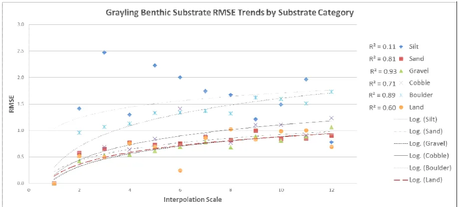
Figure 6. Little Wapiti creek substrate RMSE values with a logarithmic trend line applied showing r2 _{values for each.} In-crease in RMSE as scale moves away from the baseline reference scale shows a progressive tapering effect of accuracy loss as predictive scale moves away from the baseline. Sand substrate size maintained the smallest RMSE change between scales.

Figure 7. Grayling creek substrate RMSE values with a logarithmic trend line applied showing r2 _{values for each. Increase in} RMSE as scale moves away from the baseline reference scale shows a progressive tapering effect of accuracy loss as predic-tive scale moves away from the baseline. Sand and gravel maintained the smallest RMSE changes between scales.

variables at both sites. Decrease in spatial complexity was due in part to loss of extreme depths, flow variation and atypically located substrate variables located in the sparser data grid used for coarse scale interpolations (Figure 2). However, location and shape of deep areas, thalweg, zones of like flow, and substrate depositional areas were generally well maintained even to the termi- nal scale. Maintenance of spatial integrity is indicated by r2 _{values (percent match) from OLS regressions of each}

interpolation when compared to base scale (Table 2, Fig-

ures 8 and 9).

Wapiti Creek Residual Values at Scale 2 (top row) and Scale 12 (bottom row)

Flow Depth Substrate

Standard Deviation Categories

<−2.5 Std. Dev. −2.5 - −1.5 Std. Dev. −1.5 - −0.5 Std. Dev. −0.5 - 0.5 Std. Dev. 0.5 - 1.5 Std. Dev. 1.5 - 2.5 Std. Dev. >2.5 Std. Dev.

Figure 8. Wapiti Creek residual maps showing depth, flow, and substrate standard deviations for each of the 3630 x,y coor-dinate points at the site. Highly localized regions of standard deviation variation in scale one progress to larger regions of similar standard deviation values as scale becomes smaller, referred to in the text as a smoothing effect. Distribution pattern type of standard deviation types moves from random to clustered.

showed highly localized fluctuation in standard deviation values surrounding habitat zones with high heterogeneity and better lower standard deviation (Figures 8 and 9), while interpolations created from coarser scales saw less regional fluctuation and higher overall standard deviation from the base scale (Figures 8 and 9). Localized varia- tion in standard deviation has decreased because both maximum range of values and the amount of data used for interpolations had both decreased (Table 1). The space between each interpolated data point increased appreciably by the coarsest scale (Figure 2), which also contributed to lack of localized variation. Regressions also demonstrated models created from the coarsest scale, using 99% fewer data points and 145 times more coarse

than the original 0.11 m2_{, were able to match perform-}

ance of finer scales for some variables (Table 2).

4. Discussion

Grayling Creek Residual Value Changes between Scale 2 (row 1) and 12 (row 2)

<−2.5 Std. Dev. −2.5 - −1.5 Std. Dev. −1.5 - −0.5 Std. Dev. −0.5 - 0.5 Std. Dev. 0.5 - 1.5 Std. Dev. 1.5 - 2.5 Std. Dev. >2.5 Std. Dev. Flow

Standard Deviation Residual Classes

Depth Substrate

N

Figure 9. Grayling Creek residual maps showing depth, flow, and substrate standard deviations for each of the 3630 x,y co-ordinate points at the site. Abrupt localized changes in standard deviation are more prevalent in scale one. A more gradual change in standard deviation, or smoothing effect, may be seen in scale 12.

required to produce practical (functional, easily inter- preted, informative) maps of stream habitat. This is im- portant because adequate accuracy retention between scales affords capability for multi-scale inferences from a single data set. By defining the structure of accuracy loss of natural neighbor interpolations of stream habitat at scales other than the data collection scale through trends in RMSE and OLS regression r2, we have provided a method for estimating the amount of accuracy lost by interpolating across scales.

By observing the combined results of RMSE trends and residual values as a guide to natural neighbor inter- polative inaccuracies, it is possible to see a detailed pro- gression of errors caused by departure from initial scale when interpolating stream habitat variables. Identifying a cause for error propagation is valuable because the source of error in environmental predictive models is not always readily apparent. Maps of interpolations and re- gression residuals also aid in clarifying the scalability of stream habitat variables by showing specific locations of strong and weak model predictions when moving be- tween scales. This helps quantify what detail is elimi- nated when using data at a coarse scale, an issue impor-

tant to ecological studies [12,15,36]. The ability to un- derstand accuracy loss when interpolating at coarser scale is better understood, thus increasing the value of a single dataset.

5. Conclusion

This study indicated that the initial scale of collected data and stream size influence the range of scales at which the data set retains usefulness for predictive purposes. For instance Little Wapiti creek showed a drop in predictive accuracy below 60% at the fifth scale removed (from the original) for all habitat variables. The Wapiti site en-compassed a series of three pool/riffle zones, while Grayling creek was a single pool riffle interface (three to four times the scale of Little Wapiti). Because of stream size difference in the study, results may have identified presence of a threshold for predictive accuracy purely associated with stream size. This makes ecological sense, in which a larger order stream may have proportionally larger habitat patches which in turn maintains any scale’s predictive accuracy at further reaching scales.

scales from a single dataset was shown to be possible in this study. Spatial integrity is important because it allows accurate measurement of area of available habitat. In streams, the amount and distribution of available habitat are closely tied to species occurrence and species diver- sity, and their examination aids in ecological study at varying spatial scales [5,6,42-45].

An important question with respect to accuracy of stream habitat models, and perhaps all models, is what level of accuracy is acceptable. This paper does not at- tempt to answer that question, it only helps quantify the level of accuracy possible and identify details and accu- racy lost during the collection and analysis process. Ac- ceptable accuracy is often a function of the question be- ing asked and may vary greatly [44]. Though we do not advocate a particular level for acceptable accuracy in this study, the ability to scale a single habitat data set to a scale far removed from the original and still maintain accuracy, is a valuable tool for stream management and assessment purposes.

6. Acknowledgements

We thank Mike Strager for input on the scientific and editing processes. We thank Richard Sheehan for data collection assistance and Nicole Ten Eyck for recording of data. Reference to trade names does not imply en- dorsement of commercial products by the US govern- ment.

REFERENCES

[1] K. Looy, et al., “A Scale-Sensitive Connectivity Analysis to Identify Ecological Networks and Conservation Value in River Networks,” Landscape Ecology, Vol. 28, No. 7, 2013, pp. 1239-1249.

http://dx.doi.org/10.1007/s10980-013-9869-x

[2] D. Ruddell and E. A. Wentz, “Multi-Tasking: Scale in Geography,” Geography Compass, Vol. 3, No. 2, 2009, pp. 681-697.

http://dx.doi.org/10.1111/j.1749-8198.2008.00206.x [3] D. L. Urban, “Modeling Ecological Processes across

Scales,” Ecology, Vol. 86, No. 8, 2005, pp. 1996-2006. http://dx.doi.org/10.1890/04-0918

[4] J. T. Petty, et al., “Quantifying Instream Habitat in the Upper Shavers Fork Basin at Multiple Spatial Scales,” Proceedings of the Annual Conference of the Southeast- ern Association of Fish and Wildlife Agencies, 2001. [5] T. Petty and G. Grossman, “Patch Selection by Mottled

Sculpin (Pisces: Cottidae) in a Southern Appalachian Stream,” Freshwater Biology, Vol. 35, No. 2, 1996, pp. 261-276.

http://dx.doi.org/10.1046/j.1365-2427.1996.00498.x [6] A. R. Thompson, J. T. Petty and G. D. Grossman, “Multi-

Scale Effects of Resource Patchiness on Foraging Behav- iour and Habitat Use by Longnose Dace, Rhinichthys Ca- taractae,” Freshwater Biology, Vol. 46, No. 2, 2001, pp.

145-160.

http://dx.doi.org/10.1046/j.1365-2427.2001.00654.x [7] M. Hondzo, et al., “Estimating and Scaling Stream Eco-

system Metabolism along Channels with Heterogeneous Substrate,” Ecohydrology, Vol. 6, No. 4, 2013, pp. 679- 688.

[8] M. Wheatley and C. Johnson, “Factors Limiting Our Un- derstanding of Ecological Scale,” Ecol Complexity, Vol. 6, No. 2, 2009, pp. 150-159.

http://dx.doi.org/10.1016/j.ecocom.2008.10.011

[9] V. D. Valavanis, et al., “Modelling of Essential Fish Habitat Based on Remote Sensing, Spatial Analysis and GIS,” Hydrobiologia, Vol. 612, No. 1, 2008, pp. 5-20. http://dx.doi.org/10.1007/s10750-008-9493-y

[10] K. B. Gido, et al., “Fish-Habitat Relations across Spatial Scales in Prairie Streams,” In American Fisheries Society Symposium 48, American Fisheries Society, Bethesda, 2006.

[11] J. D. Allan, D. L. Erickson and J. Fay, “The Influence of Catchment Land Use on Stream Integrity across Multiple Spatial Scales,” Freshwater Biology, Oxford, Vol. 37, No. 1, 1997, pp. 149-161.

http://dx.doi.org/10.1046/j.1365-2427.1997.d01-546.x [12] S. A. Levin, “The Problem of Pattern and Scale in Ecol-

ogy: The Robert H. MacArthur Award Lecture,” Ecology, Vol. 73, No. 6, 1992, pp. 1943-1967.

http://dx.doi.org/10.2307/1941447

[13] J. A. Wiens, “Spatial Scaling in Ecology,” Functional Ecology, Vol. 3, No. 4, 1989, pp. 385-397.

http://dx.doi.org/10.2307/2389612

[14] A. L. Sheldon, “Cost and Precision in a Stream Sampling Program,” Hydrobiologia, Vol. 111, No. 2, 1984, pp. 147- 152. http://dx.doi.org/10.1007/BF00008627

[15] W. L. Fisher and F. J. Rahel, “Geographic Information Systems Applications in Stream and River Fisheries,” In Geographic Information Systems in Fisheries, American Fisheries Society, Bethesda, 2004, pp. 49-84.

[16] C. A. Gotway and L. J. Young, “Combining Incompatible Spatial Data,” Journal of the American Statistical Asso- ciation, Vol. 97, No. 458, 2002, pp. 632-648.

http://dx.doi.org/10.1198/016214502760047140

[17] S. D. Cooper, et al., “Implications of Scale for Patterns and Processes in Stream Ecology,” Austral Ecology, Vol. 23, No. 1, 1998, pp. 27-40.

http://dx.doi.org/10.1111/j.1442-9993.1998.tb00703.x [18] S. Gergel, et al., “What Is the Value of a Good Map? An

Example Using High Spatial Resolution Imagery to Aid Riparian Restoration,” Ecosystems, Vol. 10, No. 5, 2007, pp. 688-702.

http://dx.doi.org/10.1007/s10021-007-9040-0

[19] K. R. Sheehan and S. A. Welsh, “An Interpolation Me- thod for Stream Habitat Assessments,” North American Journal of Fisheries Management, Vol. 29, No. 1, 2009, pp. 1-9. http://dx.doi.org/10.1577/M07-080.1

[20] M. L. Stein, “Interpolation of Spatial Data: Some Theory for Kriging,” Springer, 1999.

http://dx.doi.org/10.1007/978-1-4612-1494-6

lyst,” In ArcUser, ESRI, California, 2004, pp. 32-35. [22] J. F. Kratzer, D. B. Hayes and B. E. Thompson, “Methods

for Interpolating Stream Width, Depth, and Current Ve- locity,” Ecological Modelling, Vol. 196, No. 1-2, 2006, pp. 256-264.

http://dx.doi.org/10.1016/j.ecolmodel.2006.02.004 [23] Y. Sun, et al., “Comparison of Interpolation Methods for

Depth to Groundwater and Its Temporal and Spatial Va- riations in the Minqin Oasis of Northwest China,” Envi- ronmental Modelling & Software, Vol. 24, No. 10, 2009, pp. 1163-1170.

http://dx.doi.org/10.1016/j.envsoft.2009.03.009

[24] V. Merwade, “Effect of Spatial Trends on Interpolation of River Bathymetry,” Journal of Hydrology, Vol. 371, No. 1, 2009, pp. 169-181.

http://dx.doi.org/10.1016/j.jhydrol.2009.03.026

[25] R. R. Murphy, F. C. Curriero and W. P. Ball, “Compari- son of Spatial Interpolation Methods for Water Quality Evaluation in the Chesapeake Bay,” Journal of Environ- mental Engineering, Vol. 136, No. 2, 2009, pp. 160-171. http://dx.doi.org/10.1061/(ASCE)EE.1943-7870.0000121 [26] R. J. Bennett, R. P. Haining and D. A. Griffith, “Review

Article: The Problem of Missing Data on Spatial Sur- faces,” Annals of the Association of American Geogra- phers, Vol. 74, No. 1, 1984, pp. 138-156.

http://dx.doi.org/10.1111/j.1467-8306.1984.tb01440.x [27] N. D. Le, W. Sun and J. V. Zidek, “Bayesian Multivariate

Spatial Interpolation with Data Missing by Design,” Jour- nal of the Royal Statistical Society, Series B (Methodo- logical), Vol. 59, No. 2, 1997, pp. 501-510.

[28] D. J. C. MacKay, “Bayesian Interpolation,” Neural Com- putation, Vol. 4, No. 3, 1992, pp. 415-447.

http://dx.doi.org/10.1162/neco.1992.4.3.415

[29] M. Sambridge, J. Braun and H. McQueen, “Geophysical Parametrization and Interpolation of Irregular Data Using Natural Neighbours,” Geophysical Journal International, Vol. 122, No. 3, 1995, pp. 837-857.

http://dx.doi.org/10.1111/j.1365-246X.1995.tb06841.x [30] D. Zimmerman, et al., “An Experimental Comparison of

Ordinary and Universal Kriging and Inverse Distance Weighting,” Mathematical Geology, Vol. 31, No. 4, 1999, pp. 375-390. http://dx.doi.org/10.1023/A:1007586507433 [31] A. V. Jopling and D. L. Forbes, “Flume Study of Silt

Transportation and Deposition,” Geografiska Annaler, Series A, Physical Geography, Vol. 61, No. 1-2, 1979, pp. 67-85. http://dx.doi.org/10.2307/520516

[32] I. A. Lunt, J. S. Bridge and R. S. Tye, “A Quantitative, Three-Dimensional Depositional Model of Gravelly Braided Rivers,” Sedimentology, Vol. 51, No. 3, 2004, pp. 377- 414. http://dx.doi.org/10.1111/j.1365-3091.2004.00627.x [33] B. Purkait, “Patterns of Grain-Size Distribution in Some

Point Bars of the Usri River, India,” India Journal of Sedimentary Research, Vol. 72, No. 3, 2002, pp. 367-375. http://dx.doi.org/10.1306/091001720367

[34] G. H. S. Smith and R. I. Ferguson, “The Gravel-Sand Transition along River Channels,” Journal of Sediment Research, Vol. 65, No. 2a, 1995, pp. 423-430.

[35] B. M. Weigel, et al., “Relative Influence of Variables at Multiple Spatial Scales on Stream Macroinvertebrates in the Northern Lakes and Forest Ecoregion, USA,” Fresh- water Biology, Vol. 48, No. 8, 2003, pp. 1440-1461. http://dx.doi.org/10.1046/j.1365-2427.2003.01076.x [36] N. B. Kotliar and J. A. Wiens, “Multiple Scales of Patchi-

ness and Patch Structure: A Hierarchical Framework for the Study of Heterogeneity,” Oikos, Vol. 59, No. 2, 1990, pp. 253-260. http://dx.doi.org/10.2307/3545542

[37] R. H. Waring and S. W. Running, “Forest Ecosystems: Analysis at Multiple Scales,” Elsevier, 2010.

[38] A. M. Helton, et al., “Relative Influences of the River Channel, Floodplain Surface, and Alluvial Aquifer on Si- mulated Hydrologic Residence Time in a Montane River Floodplain,” Geomorphology, 2012.

http://dx.doi.org/10.1016/j.geomorph.2012.01.004 [39] E. B. Rastetter, et al., “Aggregating Fine-Scale Ecological

Knowledge to Model Coarser-Scale Attributes of Eco- systems,” Ecological Applications, Vol. 2, No. 1, 1992, pp. 55-70. http://dx.doi.org/10.2307/1941889

[40] K. G. Boykin, et al., “A National Approach for Mapping and Quantifying Habitat-Based Biodiversity Metrics across Multiple Spatial Scales,” Ecological Indicators, Vol. 33, 2012, pp. 139-147.

[41] M. G. Wolman and A. G. Union, “A Method of Sampling Coarse River-bed Material,” Transactions of the Ameri- can Geophysical Union, Vol. 35, 1954, pp. 951-956. http://dx.doi.org/10.1029/TR035i006p00951

[42] K. O. Winemiller, A. S. Flecker and D. J. Hoeinghaus, “Patch Dynamics and Environmental Heterogeneity in Lotic Ecosystems,” Journal of the North American Ben- thological Society, Vol. 29, No. 1, 2010, pp. 84-99. http://dx.doi.org/10.1899/08-048.1

[43] C. R. Townsend, “The Patch Dynamics Concept of Stream Community Ecology,” Journal of the North Ame- rican Benthological Society, Vol. 8, No. 1, 1989, pp. 36- 50. http://dx.doi.org/10.2307/1467400

[44] C. M. Pringle, et al., “Patch Dynamics in Lotic Systems: The Stream as a Mosaic,” Journal of the North American Benthological Society, Vol. 7, No. 4, 1988, pp. 503-524. http://dx.doi.org/10.2307/1467303

[45] I. Hanski and M. E. Gilpin, “Metapopulation Dynamics,” Nature, Vol. 396, No. 6706, 1998, pp. 41-49.