Effective Task Scheduling for Embedded Systems Using Iterative Cluster Slack Optimization

http://dx.doi.org/10.4236/cs.2013.48063

Effective Task Scheduling for Embedded Systems Using

Iterative Cluster Slack Optimization

Jongdae Kim, Sungchul Lee, Hyunchul Shin

Electrical and Computer Engineering, Hanyang University, Ansan Kyeonggi-do, South Korea Email: [email protected], [email protected], [email protected]

Received August 7, 2013; revised September 7, 2013; accepted September 14,2013

Copyright © 2013 Jongdae Kim et al. This is an open access article distributed under the Creative Commons Attribution License, which permits unrestricted use, distribution, and reproduction in any medium, provided the original work is properly cited. In accor- dance of the Creative Commons Attribution License all Copyrights © 2013 are reserved for SCIRP and the owner of the intellectual property Jongdae Kim et al. All Copyright © 2013 are guarded by law and by SCIRP as a guardian.

ABSTRACT

To solve computationally expensive problems, multiple processor SoCs (MPSoCs) are frequently used. Mapping of applications to MPSoC architectures and scheduling of tasks are key problems in system level design of embedded sys- tems. In this paper, a cluster slack optimization algorithm is described, in which the tasks in a cluster are simultaneously mapped and scheduled for heterogeneous MPSoC architectures. In our approach, the tasks are iteratively clustered and each cluster is optimized by using the branch and bound technique to capitalize on slack distribution. The proposed static task mapping and scheduling method is applied to pipelined data stream processing as well as for batch process- ing. In pipelined processing, the tradeoff between throughput and memory cost can be exploited by adjusting a weight- ing parameter. Furthermore, an energy-aware task mapping and scheduling algorithm based on our cluster slack opti- mization is developed. Experimental results show improvement in latency, throughput and energy.

Keywords: Multi-Processor; Mapping; Scheduling

1. Introduction

As many systems in communication and multi-media be- come more and more complex and require a large amount of computation, a single processor can’t frequently sat-isfy the performance criteria. Since designing a high per-formance custom integrated circuit requires great cost and a long design period, using multiple processors (or multi-cores) is increasingly seen as an alternative ap-proach. However, mapping of applications to MPSoC ar- chitectures and scheduling of tasks are key problems in high-level design of embedded systems.

System performance or throughput can be improved by using parallel processing or pipelining. In parallel pro- cessing, multiple functions can be executed in parallel or a single function can be executed for multiple data sets. In pipelining, consecutive data streams are processed with overlaps in processing time for larger throughput. Data streams of audio and video signals should be proc- essed within appropriate interval between consecutive inputs to provide the correct information for users. The most important factor to decide the performance of a pi- peline is the interval between the consecutive inputs, and

this interval can be fixed or varied. A small interval means a higher throughput.

Mapping and scheduling problems for multiple proc- essors belong to the class of NP-hard problems [1]. Re- search has been carried out in solving task mapping and scheduling problems. Different tools and models have been developed to address the problems above.

The branch and bound algorithm can be used to map an application to architecture so that the total execution time is minimized. This algorithm checks all possible cases of assignments of n tasks to m processors leading to huge search space and minimizes the search area by using bounding procedure to reach an optimum solution in less time [2]. However, due to the worst-case expo-nential complexity, this method can only be used for “small” sized problems.

2. Related Works

elements (PEs). The mapping has to be found under con- straints where all tasks are assigned to PEs and every task is assigned to only one PE. The task scheduling problem is the problem of assigning the order of tasks in the system to optimize the overall performance for the given application.

A very popular heuristic method to schedule tasks is list scheduling [3]. Tasks are scheduled from a prespeci- fied list and the task with the highest priority is re- moved from the priority list and then scheduled, one by one.

For scheduling heterogeneous processing elements, the Heterogeneous Earliest Finish Time (HEFT) algorithm [4] is used. This algorithm uses upward rank value which represents the longest path from each task to set the pri- ority of each task. The task list is ordered by decreasing value of upward rank. Based on this list, tasks are sched- uled onto the processors that have the earliest finish time. Another scheduling algorithm based on list scheduling is the Critical-Path-On a Processor (CPOP) algorithm [4]. In contrast to the HEFT algorithm, this algorithm uses upward ranking and downward ranking to set the priority of each task. The downward ranking is computed by adding the average execution time of the task and maxi- mum downward rank value of the predecessors. The task with highest priority is selected for execution. If the se- lected task is on a critical path, then it is scheduled for the critical path processor. A critical processor is one that minimizes the cumulative computation cost of the tasks on the critical path. Otherwise, the task is assigned to the processor which has the minimum execution finish time of the task.

Similarly, Performance Effective Task Scheduling (PETS) algorithm [5] consists of three stages, Level sorting, Task prioritization, and Processor selection. In Level sorting, each task is sorted at each level in order to group the tasks. Because of this, tasks in the same level could be executed in parallel. In Task prioritization, the priority of each task is computed by using average computation cost, data transfer cost, and highest rank of the predecessors. In Processor selection, task is assigned to the processor which gives the minimum finish time. Compared to the Heft and CPOP algorithm, PETS algorithm shows good performance.

The force-directed scheduling algorithm [6] prioritizes and schedules the subtasks based on the resource utilize- tion probability in each step. Recently, other techniques, such as simulated evolution based method [7], were re- ported. The genetic algorithm [8,9] is a widely re- searched random search technique. This algorithm exe- cutes in generations, producing better solutions using crossover and mutation operators. In the genetic algo- rithm, candidate solutions are represented by sequences of symbols called chromosomes. Evolutionary algori-

thms (EAs) operate on a population of potential solu- tions, applying the principle of survival of the fittest to produce successively better approximations to a solution. At each generation of the EAs, a new set of approxima- tions is created by the process of selecting individuals according to their level of fitness in the problem domain and reproducing them using variation operators. This process may lead to the evolution of populations of indi- viduals that are better suited to their environment than the individuals from which they were created, just as in natural adaptation. EAs are characterized by the repre- sentation of the individual, the evaluation function rep- resenting the fitness level of the individuals, and the population dynamics such as population size, variation operators, parent selection, reproduction and inheritance, survival competition method, etc. To have a good bal- ance between exploration and exploitation, those com- ponents should be designed properly [10].

Like all other EAs, a quantum-inspired evolutionary algorithm (QEA) also consists of the representation of individuals, the evaluation function, and the population dynamics. The only difference is that it uses quantum bits as probabilistic representation for individuals instead of binary representation of genes [7].

In [11], energy aware scheduling that uses task order- ing and voltage scaling in an integrated manner is pre- sented, and the voltage level instead of the speed level was considered in the cost function for each processor. Dynamic voltage scaling (DVS) is one of the most pow- erful techniques to reduce energy consumption [12,13]. All these methods are heuristic approaches.

3. Mapping and Scheduling for Batch

Processing Systems

By using the branch and bound algorithm [2], one can obtain an optimum solution for “small” mapping prob- lems. However, one cannot afford run-time (CPU time) for large problems due to the exponential worst case run-time. To solve the complex mapping problems in a reasonable time, we propose a cluster slack optimization algorithm. In this algorithm, we divide all tasks in a task flow graph by a given number of clusters. Each cluster is optimized to find a best solution capitalizing on the slack distribution. The algorithm to minimize the execution (finish) time can be written as in Algorithm 1.

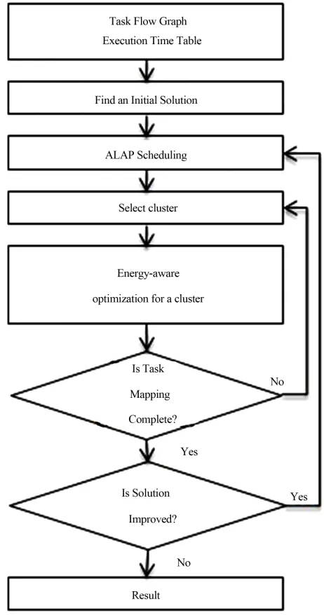
The cluster slack optimization algorithm consists of five major steps, which are initialization, As Late As Possible (ALAP) scheduling, making clusters, cluster selection, and slack optimization for the selected cluster.

Algorithm 1. Cluster slack optimization algorithm for task mapping and scheduling.

Input : task flow graph, execution time table, processors Output : mapped and scheduled tasks

Find an initial greedy solution;

while ( solution can be improved ) do

ALAP scheduling for slack maximization; Make clusters;

while ( not completed ) do Select a cluster to optimize;

Find the task optimization zone for the selected cluster;

Optimize the tasks in the selected cluster within the task optimization zone;

end end

Output the solution;

clustering the given tasks into several clusters in making cluster step, only a small number of tasks in a cluster are remapped and re-scheduled, and thus the run-time can be controlled by adjusting the cluster size. In the cluster selection step, an un-processed task cluster is selected in order of execution start times. In the optimization step, we optimally remap and reschedule the tasks in the se- lected cluster within the task optimization zone. The task optimization zone is defined by two boundaries called floor and ceiling. When the optimization of the current cluster is finished, the floor and the ceiling will be up- dated and thus the task optimization zone is moved. The optimization is repeated when the new solution is better than the previous best solution.

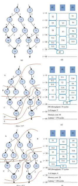
Figure 1 shows an example from [5], in which 10

tasks are to be mapped to 3 heterogeneous processors. Figure 1(a) shows the task flow graph and Figure 1(b) shows the execution time table from [5]. For example, the execution of task T1 by processor P1 takes 14 cycles. The communication time to transfer the output of task 1 to the input of task 2 takes 18 cycles as shown by the edge weight. Different processors may take different number of cycles to finish a given task. Figures 1(c)-(e) show the scheduling results by using the HEFT, CPOP and PETS algorithm respectively [5]. The produced solu- tions use 80, 86, and 79 cycles, respectively.

Now we explain our method by using the same exam- ple. Figure 2(a) shows the initial solution by using greedy list scheduling and Figure 2(b) shows the solu- tion after the ALAP scheduling step. The produced initial solution used 82 cycles.

After the ALAP scheduling step, all tasks are clustered in the order of execution start time, and each cluster is re-mapped and re-scheduled. We perform the branch and bound by evaluating the slacks of all possible mappings and schedules for tasks in the current cluster. The object- tive of slack optimization is to maximize the minimum slack for each processor. Slack optimization tries to achieve a near global optimum solution by solving itera- tive local optimization problems. Figure 3 shows an ex- ample process of slack calculation. Let STi be starting

time of task i and FTi be finishing time of task i. Let Ca,b

be communication time from na to nb and Ei,j be execu-

tion time of task i on processor j. Since na, ni, and nd are

executed on P1, the communication times Ca,i and Ci,d

can be 0. Now, we define the slack when the task ni is

mapped to P1, as follows.









, , ,1 ,

, , ,1 ,

{max , },

Slack min

{max , }

d a a i b b i i

i

f a a i b b i i

ST FT C FT C ET C

ST FT C FT C ET C

                   i d i f

The goal of the optimization is to remap/re-schedule to maximize the slack, since the minimum slack of all out- put tasks in the current cluster is the gain of the optimi- zation. In other words, the latency can be reduced by the minimum slack.

Figure 4 shows the process of our algorithm for the example shown in Figure 1. After ALAP scheduling, all tasks are clustered to form 3 clusters as shown in Figure 4(a). In this case, 1st_cluster = {n1, n2, n4, n5}, 2nd_cluster = {n3, n6, n7}, and 3rd_cluster = {n8, n9, n10}. Figures 4(b)-(d) show optimized results after op-timization of each cluster. In Figure 4(b), the slacks of each processor are 13, 19, and 7 cycles, respectively. So we can reduce 7 cycles after the 1st cluster optimization. In Figure 4(c), there is no change during the 2nd cluster optimization. In the same way, we can reduce 1 cycle after the 3rd cluster optimization. Finally, the solution is

reduced to 74 cycles, and 8 cycles are reduced when compared to the initial solution. This is really the opti- mum solution, as verified by using the branch and bound algorithm. Compared to the three previous algorithms shown in Figure 1, our new iterative slack optimization algorithm produced a significantly better solution (the latency has been reduced to 74 cycles from 79 cycles or more), which is the optimum solution in this case.

4. Mapping and Scheduling of Pipelined

Systems for Data Stream Processing

4.1. Throughput Increase by Pipelining

Figure 1. An example and scheduling results. (a) Task flow graph; (b) Execution time table; (c) The HEFT algorithm [4]; (d) The CPOP algorithm [4] (e) The PETS algorithm [5].

Figure 2. (a) Initial solution by using list scheduling; (b) So- lution after the ALAP scheduling.

show the data communication times. Different processors may take different numbers of cycles to finish a given task.

In batch-mode task parallel execution, the goal is to minimize latency. However, continuous data stream processing is needed to process audio and video signals. Therefore, the most important factor of scheduling for data stream processing is to reduce the interval between

Figure 3. Calculation of the slack.

consecutive data inputs for larger throughput. A small interval means higher throughput. To reduce data input interval (DII), we divide all tasks into several stages and use pipelining. For example, three candidate schedule positions of task 5 (T5) of the task flow graph shown in Figure 5(a) are shown in Figure 6(a) for the batch-mode task parallel execution. For pipelined execution, data can be processed by forming several stages. When the first stage processes i-th input data, the second stage process (i-1)-th input data. This pipelined scheduling allows 7 candidates schedule positions for T5, as shown in Figure 6(b).

4.2. Optimization Using a Cost Function

Usually, the throughput can be increased by increasing the number of stages. However, this may increase the latency and memory cost. To optimize the trade-off, we define the following cost function.





Total _ Cost DII _ cost   1  Memory _ cost (1)

Figure 4. (a) Task clustering after ALAP scheduling; (b) Result after 1st cluster optimization; (c) Result after 2nd

cluster optimization; (d) Result after 3rd cluster optimiza-

tion.

(a) (b)

Figure 5. (a) Task flow graph with 15 tasks; (b) Execution time table for 3 processors (P1, P2, P3).

be computed as follows.



Memory_cost N

i i

i



M S







where N is the number of stages, Mi is the amount of memory for i-th stage, and Si is the number of pipeline stages to store the data of i-th stage.

Figure 7 shows the pipelined schedule results of the

(a) (b)

Figure 6. (a) Candidate schedule positions of T5 in batch- mode execution; (b) Candidate schedule positions of T5 in pipelined execution.

task flow graph given in Figure 5. The clustering results are shown in Figures 7(b) and (c) when α = 0.7 and α = 0.3, respectively. Five stages (A, B, C, D, E) are used when α = 0.7 as shown in Figure 7(b) and four stages (A, B, C, D) are used when α = 0.3 as shown in Figure 7(c). The result of batch processing is shown in Figure 7(d), in which the data input interval (DII) is 49. Figure 7(e) shows the pipelined schedule using 5 stages with DII of 34.

When the number of stages is 5, the latency can be up to 5× DII (5 × 34 = 170 cycles), even though one set of input data can be processed every 34 cycles. Figure 7(f) shows the pipelined schedule using 4 stages with DII of 37. When the number of stages is 4, the latency can be up to 4× DII (4 × 37 = 148 cycles). Memory_cost is 44 and 28 when α is 0.7 and 0.3, respectively. When α is small then the weight of Memory_cost in (1) is large and thus memory cost is reduced even though DII can be in- creased. This shows that α can be used to optimize the trade-off between DII and memory cost. Figure 8 shows how the data streams flow through the pipelining stages.

5. Energy Aware Mapping and Scheduling

Over the last decade, manufacturers have competed to advance the performance of processors by raising the clock frequency. However, recent computer systems are focused on battery-driven devices such as portable handheld devices, sensors, and robots, rather than tradi- tional large devices and desktops. Therefore, technical issues are miniaturization and low energy consumption. Specially, low power is extremely important for many real-time embedded systems. To apply our iterative slack optimization algorithm for energy aware mapping and scheduling, we only need to modify the cost function in slack optimization. The modified cost we used is shown in (3).The energy-aware cluster slack optimization algo- rithm is shown in Figure 9.





E

Figure 8. Processing procedure of an input data stream.

where β is the weighting factor and K is the scaling con-stant.

6. Experimental Results

We implemented the cluster slack optimization algorithm by using the “C” programming language under the Win- dows operation system. The experiments were performed by using both real applications and randomly generated task flow graphs with 20 to 100 tasks. The parallel Gaus- sian elimination, LU decomposition [9] and molecular dynamics [14] are used as real applications. The tasks are mapped and scheduled by our method and by branch and bound, HEFT [4], CPOP [4] and PETS [5] algorithms for comparisons.

Table 1 shows the solution comparisons for real ap- plications. A base algorithm for comparisons is the branch and bound algorithm which can find an optimum solution by spending much more time than other algo- rithms.

However, in molecular dynamics applications, we use our algorithm as a base algorithm because the branch and bound algorithm cannot obtain the solution within 24 hours.

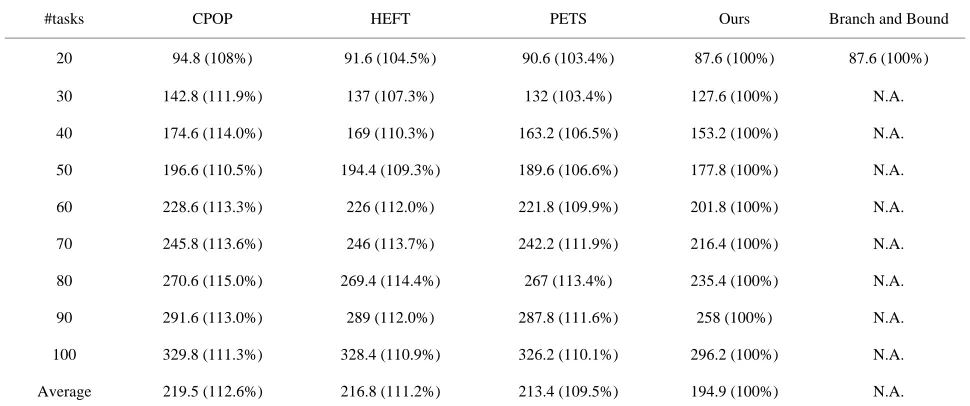
Table 2 shows the solution comparisons for the ran- domly generated task flow graphs. In experiments, we used 5 randomly generated task graphs for each number of tasks (# tasks). The results of our algorithm are ob- tained by taking up to 20 tasks in a cluster.

Randomly generated task graphs with 20 to 50 tasks are used for experiments in pipelined systems. The re- sults are compared with those of a recent method, QEA [7]. Table 3 shows DII_cost and Memory cost for QEA and our method. In Equation (1), α = 0.7 was used. On

Figure 9. Energy aware cluster optimization algorithm.

the average, our method shows better results. DII_cost is improved by 2% and Memory_cost is improved by 23%.

Table 4 shows tradeoff between DII_cost and Mem- ory_cost by changing the weight α. As α gets smaller, DII increases and Memory_cost decreases.

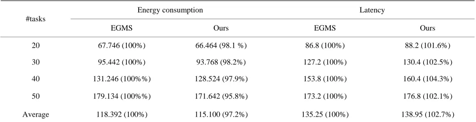
Energy aware mapping and scheduling experiments are processed by using randomly generated task flow graphs with 20 to 50 tasks. We use three commercial processor power models consisting of XScale, PowerPC, and DSP [15] for power estimation. The tasks are mapped and scheduled by using our method and the re- sults are compared with those of Energy Gradient-based Multiprocessor Scheduling (EGMS) [11].

Table 1. Solution comparisons for real applications.

#tasks CPOP HEFT PETS Ours Branch and Bound

Parallel Gaussian elimination (15 tasks) 120.7% 112.2% 109.7% 100% 100%

LU decomposition (14 tasks) 113.1% 111.9% 103.5% 100% 100%

Molecular dynamics (40 tasks) 120.4% 117.6% 109.6% 100% N.A.

Table 2. Solution comparisons for randomly generated task flow graphs with 20 to 100 tasks.

#tasks CPOP HEFT PETS Ours Branch and Bound

20 94.8 (108%) 91.6 (104.5%) 90.6 (103.4%) 87.6 (100%) 87.6 (100%)

30 142.8 (111.9%) 137 (107.3%) 132 (103.4%) 127.6 (100%) N.A.

40 174.6 (114.0%) 169 (110.3%) 163.2 (106.5%) 153.2 (100%) N.A.

50 196.6 (110.5%) 194.4 (109.3%) 189.6 (106.6%) 177.8 (100%) N.A.

60 228.6 (113.3%) 226 (112.0%) 221.8 (109.9%) 201.8 (100%) N.A.

70 245.8 (113.6%) 246 (113.7%) 242.2 (111.9%) 216.4 (100%) N.A.

80 270.6 (115.0%) 269.4 (114.4%) 267 (113.4%) 235.4 (100%) N.A.

90 291.6 (113.0%) 289 (112.0%) 287.8 (111.6%) 258 (100%) N.A.

100 329.8 (111.3%) 328.4 (110.9%) 326.2 (110.1%) 296.2 (100%) N.A.

Average 219.5 (112.6%) 216.8 (111.2%) 213.4 (109.5%) 194.9 (100%) N.A.

Table 3. DII and memory cost comparisons in pipelined systems.

DII cost Memory cost

#tasks

QEA Ours QEA Ours

20 425 101.9%) 417 (100%) 8910 (128.7%) 6920 (100%)

30 831 (101.3%) 820 (100%) 15,353 (122.1%) 12,568 (100%)

40 1241 (102.8%) 1207 (100%) 19,181 (122.9%) 15,599 (100%)

50 1616 (102.3%) 1579 (100%) 23,926 (123.1%) 19,434 (100%)

Total 4113 (102.2%) 4023 (100%) 67,370 (123.6%) 54,521 (100%)

Table 4. Trade off between DII and memory.

α = 0.7 α = 0.5 α = 0.3

#tasks

DII Memory DII Memory DII Memory

20 417 6920 459 6327 489 5967

30 820 12,568 907 11,397 967 10,994

40 1207 15,599 1331 13,151 1481 11,831

50 1579 19,434 1781 17,924 1861 15,984

Table 5. Energy consumption and latency comparisons (β = 0.3).

Energy consumption Latency

#tasks

EGMS Ours EGMS Ours

20 67.746 (100%) 64.974 (95.9%) 86.8 (100%) 91.2 (105.1%)

30 95.442 (100%) 90.238 (94.5%) 127.2 (100%) 131.8 (103.6%)

40 131.246 (100%) 127.344 (97.0%) 153.8 (100%) 161.2 (104.8%)

50 179.134 (100%) 163.128 (91.1%) 173.2 (100%) 179.4 (103.6%)

Average 118.392 (100%) 111.421 (94.1%) 135.25 (100%) 140.90 (104.2)

Table 6. Energy consumption and latency comparisons (β = 0.7).

Energy consumption Latency

#tasks

EGMS Ours EGMS Ours

20 67.746 (100%) 66.464 (98.1 %) 86.8 (100%) 88.2 (101.6%)

30 95.442 (100%) 93.768 (98.2%) 127.2 (100%) 130.4 (102.5%)

40 131.246 (100%%) 128.524 (97.9%) 153.8 (100%) 160.4 (104.3%)

50 179.134 (100%%) 171.642 (95.8%) 173.2 (100%) 176.8 (102.1%)

Average 118.392 (100%) 115.100 (97.2%) 135.25 (100%) 138.95 (102.7%)

ments, we used 5 randomly generated task graphs for each task.

The results of our algorithm are obtained by taking up to 20 tasks in a cluster for simultaneous optimization.

7. Conclusions

We developed an effective algorithm to map and sched-ule tasks simultaneously for heterogeneous processors. By partitioning all tasks into several clusters, only a small number of tasks in a cluster are re-mapped and re- scheduled at the same time. Therefore, the run-time can be controlled by adjusting the cluster size and can in- crease linearly with the number of tasks. Experimental results show that our algorithm can obtain 9.5%, 11.2% and 12.6% better solutions compared to PETS, HEFT and CPOP algorithms, respectively, in batch-mode sys- tems. Furthermore, our method can improve the DII_cost by 2% and Memory_cost by 23% when compared to [7] in pipelined systems. Finally, energy-aware cluster slack optimization results show that our algorithm can effect- tively perform the trade-off between the latency and the energy consumption.

The techniques described in this paper can be applied to static scheduling for multiple processors, to optimize latency, throughput and energy. Future works include developing dynamic scheduling techniques, optimization for networks on chip and consideration of memory band- width.

8. Acknowledgement

This work was supported by the Ministry of Science, ICT & Future Planning and IDEC Platform center (IPC) in Korea.

REFERENCES

[1] P. Luh, D. Hoitomt, E. Max and K. Pattipati, “Schedule Generation and Reconfiguration for Parallel Machines,”

Robotics and Automation, Vol. 6, No. 6, 1990, pp. 687- 696. http://dx.doi.org/10.1109/70.63271

[2] K. Vivekanandarajah and S. Pilakkat, “Task Mapping in Heterogeneous MPSoCs for System Level Design,” 13th

IEEE International Conference on Engineering of Com- plex Computer Systems, Belfast, 31 March 2008-3 April 2008, pp. 56-65.

[3] T. Adams, K. Chandy and J. Dickson, “A Comparison of List Schedules for Parallel Processing Systems,” Com-

munications of the ACM, Vol. 17, No. 12, 1974, pp. 685- 690. http://dx.doi.org/10.1145/361604.361619

[4] H. Topcuoglu, S. Hariri and M. Wu, “Performance-Ef- fective and Low-Complexity Task Scheduling for Het- erogeneous Computing,” IEEE Transactions on Parallel

and Distributed Systems, Vol. 13, No. 3, 2002, pp. 260- 274.

[5] E. Ilavarasan and P. Thambidurai, “Low Complexity Per- formance Effective Task Scheduling Algorithm for Het- erogeneous Computing Environments,” Journal of Com-

puter Sciences, Vol. 3, 2007, pp. 94-103.

Algo-rithms for High-Level Synthesis,” 26th Conference on

Design Automation, 25-29 June 1989, pp. 1-6. http://dx.doi.org/10.1145/74382.74383

[7] H. Yang and S. Ha, “Pipelined Data Parallel Task Map- ping/Scheduling Technique for MPSoC,” Proceedings of

Design, Automation & Test in Europe Conference & Ex- hibition, Nice, 20-24 April 2009, pp. 69-74.

[8] A. Wu, H. Yu, S. Jin, L. Kuo-Chi and G. Schiavone, “An Incremental Genetic Algorithm Approach to Multiproc-essor Scheduling,” IEEE Transactions on Parallel and

Distributed Systems, Vol. 15, No. 9, 2004, pp. 824-834. http://dx.doi.org/10.1109/TPDS.2004.38

[9] T. Tsuchiya,T. Osada and T. Kikuno, “Genetic-Based Mul- tiprocessor Scheduling Using Task Duplication,”

Micro-processors and Microsystems, Vol. 22, 1998, pp. 197-207. http://dx.doi.org/10.1016/S0141-9331(98)00079-9

[10] K. Han and J. Kim, “Quantum-Inspired Evolutionary Al- gorithm for a Class of Combinatorial Optimization,”

IEEE Transactions on Evolutionary Computation, Vol. 6, No. 6, 2002, pp. 580-593.

http://dx.doi.org/10.1109/TEVC.2002.804320

[11] L. Goh, B. Veeravalli and S. Viswanathan, “Design of Fast and Efficient Energy-Aware Gradient-Based Sched-uling Algorithms Heterogeneous Embedded Multiproc-essor Systems,” IEEE Transactions onParallel and

Dis-tributed Systems, Vol. 20, No. 1, 2009, pp. 1-12. [12] Y. Yu and V. Prasanna, “Energy-Balanced Task

Alloca-tion for Collaborative Processing in Wireless Sensor Net- works,” Mobile Networks and Applications, Vol. 10, 2005, pp. 115-131.

http://dx.doi.org/10.1023/B:MONE.0000048550.31717.c 5

[13] A. Andrei, M. Schmitz, P. Eles, Z. Peng, B. M. Al- Hashimi, “Overhead-Conscious Voltage Selection for Dy- namic and Leakage Energy Reduction of Time-Cons- trained Systems,” IEE Proceedings on Computers and

Digital Techniques, Vol. 152, No. 1, 2005, pp. 28-38. http://dx.doi.org/10.1049/ip-cdt:20045055

[14] S. Kim and J. Browne, “A General Approach to Mapping of Parallel Computation upon Multiprocessor Architec-tures,” Proceedings of the International Conference on

Parallel Processing, 1988, pp. 1-8.

[15] G. Zeng, T. Yokoyama, H. Tomiyama and H. Takada, “Practical Energy-Aware Scheduling for Real-Time Mul-tiprocessor Systems,” 15th IEEE International