http://dx.doi.org/10.4236/ojs.2016.62029
Comparison of Two Sample Tests Using Both
Relative Efficiency and Power of Test
Edith Uzoma Umeh, Nkiru Obioma Eriobu
Department of Statistics, Nnamdi Azikiwe University, Awka, Nigeria
Received 1 February 2016; accepted 24 April 2016; published 27 April 2016
Copyright © 2016 by authors and Scientific Research Publishing Inc.
This work is licensed under the Creative Commons Attribution International License (CC BY). http://creativecommons.org/licenses/by/4.0/
Abstract
This paper, comparison of two sample tests, is motivated by the fact that in the test of significant difference between two independent samples, numerous methods can be adopted; each may lead to significant different results; this implies that wrong choice of test statistic could lead to erro-neous conclusion. To prevent misleading information, there is a need for proper investigation of some selected methods for test of significant difference between variables/subjects most espe-cially, independent samples. The paper examines the efficiency and sensitivity of four test statis-tics to ascertain which test performs better. Based on the results, the relative efficiency favours median test as being more efficient than modified median test for both symmetric and asymmetric distributions. In terms of power of test, median test is more sensitive than Modified Median (MMED) test since it has higher power irrespective of the sample sizes for both symmetric and asymmetric distribution. In terms of relative efficiency for asymmetric distribution Modified Mann- Whitney U test is more efficient than Mann-Whitney U test (MMWU), and then for symmetric dis-tribution, Mann-Whitney U test (MMWU) is more efficient than Modified Mann-Whitney in sample size of 5; but for other sample sizes considered Modified Mann-Whitney U test (MMWU) is better than Mann-Whitney. Using power of test for both symmetric and asymmetric distributions, Mann- Whitney is more sensitive than Modified Mann-Whitney U test (MMWU) because it has higher power.
Keywords
Asymmetric, Symmetric, Nonparametric Test, Two Sample Tests, Power of Test, Relative Efficiency
1. Introduction
possible assumptions that might have been made to enable the use of such methods. Numerous methods exist for testing statistical hypotheses in various conditions. In some cases, the probability distribution of the population from which samples are drawn is known. For instance, if the population is assumed to be normal; then, the sam-ple size is assumed to be sufficiently large to justify the assumption of normality. In special cases, the samsam-ple sizes are very small and the probability distribution of the populations from which samples are drawn is un-known; hence, the sample is said to be distribution free and only non-parametric methods are applied. Thus, in most cases where the assumption of parametric methods is violated or not met, the non-parametric methods are usually preferred. Non-parametric methods that readily suggest themselves include the Median and the Mann- Whitney U test [1]. These methods require that the populations from which the samples are drawn to be con-tinuous so that the probability of obtaining tied observations is at least theoretically zero [2]. Statistical tests could be for either paired or unpaired. In a paired test (Matched sample test), the data are collected from subjects measured at two different points wherein each subject has two measurements which are done before and after the treatment. Unpaired test on the other hand is when data are collected from two different and independent subjects. The size of the two samples may be equal or not, depending on the requirement of the test statistic. Techniques or methods for performing two sample tests abound but the question is “which method(s) perform better and under what conditions do they perform better when dealing with independent samples?” To make an articulate attempt to answer these questions, there is a need for proper and adequate comparative study of similar methods that can be used for the purpose of interest. The methods/techniques are: median test, modified median test intrinsically adjusted for ties, Mann-Whitney U test and modified intrinsically ties adjusted Mann-Whitney U test. All the above listed methods are for test of significant difference between variables/subjects when having independent samples. Wide comparison would expose researchers to conditions under which the methods are used to prevent type I or type II errors. In statistical computation, test statistics sometimes are affected by nature of data; that is, the distribution of the data which could be either symmetric or asymmetric in nature. In the de-termination of more effective statistical method, not just the null hypothesis should be of paramount interest but also the alternative hypothesis which implies that power of test plays an important role in the determination of effectiveness of statistical methods. The maximum value of power of test is 1 and the least is zero which is non- negativity property. The higher the power of test, the better the method and the lower the value, the less effec-tive the method. In this paper, methods of analyzing two independent samples drawn from independent popula-tions would be considered by subjecting some set of data to different condipopula-tions, such as sample size, to deter-mine the condition under which they perform optimally in terms of Relative Efficiency (R.E) and power. The power efficiency of median test decreases as the sample sizes increases reaching an eventual asymptotic effi-ciency of 2π [3]. The modified median test intrinsically adjusted for ties was compared with the existing technique, ordinary median test; and the conclusion was that the modified median test intrinsically adjusted for ties easily enables the isolation of tied observations and estimation of their probability of occurrence [2].
2. Material and Methodology
(1) MEDIAN TEST: Median test is a procedure for testing whether two independent groups (samples) differ in central tendencies represented by the population median [4]. The null hypothesis is
0: 0
H π+ =θ Vs H1:π+≠θ0 (1)
where θ =0 0.5. The test statistic is
(
)
( )
(
(
)
)
2 2
1 2 0
1 2 0 2 1 ˆ ˆ ˆ var n n
W n n
W θ π π π θ χ + + + − − = = − ⋅ (2)
which under H0 becomes
(
)
(
)
2 1 2
2 ˆ 0.
ˆ
5 . ˆ 1 n n π
π π χ + + + − =
− (3)
(2) Modified median test intrinsically adjusted for ties is used for test of equality in population media [2]. The null hypothesis H0:M1=M2=M is equivalent to the null hypothesis,
0:
H π+ =π− or H0:π+−π−=0 (4)
1: 0.
H π+−π−≠
The test statistic is
(
)
2 2 2 w w mn mn χπ+ π− =
+ −
(5)
where
. w= f+− f−
m is sample size of variable X. n is sample size of variable Y.
0
, ,
π π π+ −
are respectively the probabilities that observations or scores by subjects from population X are on the average greater than , equal to, or less than observations or score by subjects from population Y.
0 , ,
f+ f f− are respectively the number of 1’s, 0’s and −1’s in the frequency distribution of these mn values of Uij.
Reject H0 at α-level of significance if
2 2 1α;1
χ
≥χ
− , otherwise, accept.(3) Mann-Whitney U test is used for determination of the likelihood that two samples/groups emanated from the same population/distribution [5].
The test statistic is
. u u U Z µ σ −
= (6)
Then,
(
)
1 1
1 2 1
1 2
n n
U=n n + + −R (7)
where
n1 is the total number of the first group/observation. n2 is the total number of the first group/observation. R1 is the sum of the ranks for the first group/observation. Then
1 2 2 U
n n
µ = (8)
is the mean and
(
)
1 2 1 2 1
12
u
n n n n
σ = + + (9)
is the standard deviation.
This Z-score is, as usual, compared at a given level of significance with an appropriate critical value obtained from a normal distribution table for a rejection or acceptance of the null hypothesis.
(4) Modified Intrinsically Ties Adjusted Mann-Whitney U test is used to check whether two samples could have been drawn from the same population/distribution [6].
The test statistic is
( )
(
2 2(
2. 1)
(
1. 2)
(
)
)
2. 1 1. 2 1
2 2 2 2 2 . . 2 . var .
n R n R
n R R R R
w
w n
χ
π π π π
∗ ∗ + − + −
= =
+ + − −
−
where
n1 is the sample size of variable x1. n2 is the sample size of variable x2.
R1 and R2 are the respectively sums of the ranks assigned to observations from populations x1 and x2 in the combined ranking of these observations from the two populations.
π+
, π− are respectively the probabilities that observations or scores by subject from population X1 is on the average greater than or less than observations or scores by subject from population X2.
The test hypothesis will be
0: 0
H π+−π−= vs
1: 0
H π+−π−≠ .
Reject H0 at α-level of significance if
2 2 1α;1
χ
≥χ
− ; otherwise, accept.Relative Efficiency of two test statistics (R.E) is the ratio of the variances of one of the two test statistics to the other (say: T1 to T2) for equal sample size n. That is, relative efficiency of test T2 to T1 is defined as
(
)
( )
( )
1 2 12 v
R. ar
var
E T T; T
T
= . (11)
Between test 1 and test 2, test 2 is relatively more efficient than test 1 if the relative efficiency of the tests,
(
2 1)
R.E T T; is at least unity; that is if R.E
(
T T2; 1)
≥1 and hence test T2 is said to be more powerful than test 1T.
Power of a statistical test is the probability of rejecting the null hypothesis when it is in fact false and should be rejected (i.e. the probability of not committing a type II error [7]. In other words, the power of test is equal to 1−
β
, which is also known as the sensitivity [8]; whereβ
is the probability of committing type II error = error rate. Error rate is defined as the ratio of number of erroneous decision to number of replicate. That is;(
)
Number of error output No of trials Repli .R
e E
cat
= .
In this paper, Monte Carlo’s Simulation techniques was used in the generation of data of different distribu-tions and varying sample sizes ranging from 5 to 100 which was repeated 30 times for each sample size. In the simulation, sample size of 5, 10, 50 and 100 were considered to cover both small and large sample sizes. Monte Carlo simulation is defined as a method to generate random sample data based on some known distribution for numerical experiments. Monte Carlo simulation is an algorithm used to determine performance of an estimator or test statistic under various scenarios [9].
3. Algorithm for Monte Carlo Simulation
1) Specify the data generation process.2) Choose a sample size N for the MC simulation.
3) Choose the number of times to repeat the MC Simulation.
4) Generate a randomsample of size N based on the data generation process. 5) Using random sample generated in 4 above, calculate the test statistic(s). 6) Go backto (4) and (5) until desirable replicate is achieved.
7) Examine parameter estimates, test statistics, etc.
In the paper, for data from a known family of distributions, Gamma (4, 0.3) and Beta (2, 2) were used.
4. Result
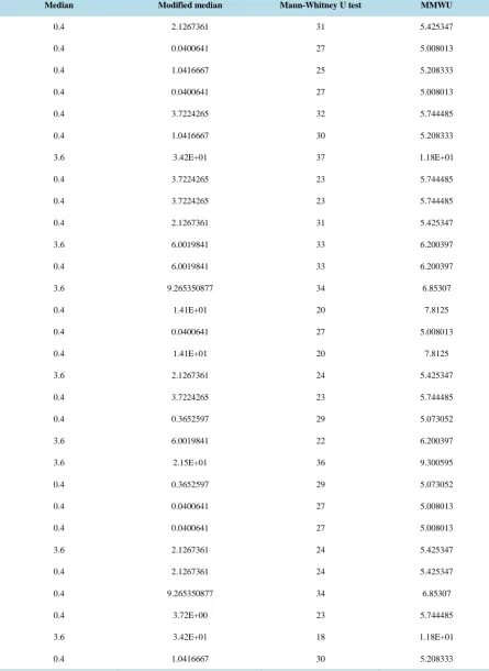
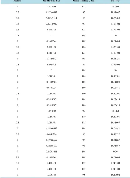
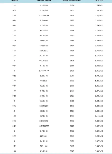
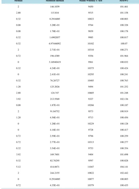
From the simulated data using Monte Carlo simulation approach, the following results were obtained: Tables 1-4 are test statistics value of asymmetric distribution for different sample size while Tables 5-8 are test statis-tics value of symmetric distribution for different sample size. Table 9 is the variance of the test statistic consid-ered. Table 9 is calculated from Tables 1-8.
Table 1. Test statistic value of sample size 5.
Median Modified median Mann-Whitney U test MMWU
0.4 2.1267361 31 5.425347
0.4 0.0400641 27 5.008013
0.4 1.0416667 25 5.208333
0.4 0.0400641 27 5.008013
0.4 3.7224265 32 5.744485
0.4 1.0416667 30 5.208333
3.6 3.42E+01 37 1.18E+01
0.4 3.7224265 23 5.744485
0.4 3.7224265 23 5.744485
0.4 2.1267361 31 5.425347
3.6 6.0019841 33 6.200397
0.4 6.0019841 33 6.200397
3.6 9.265350877 34 6.85307
0.4 1.41E+01 20 7.8125
0.4 0.0400641 27 5.008013
0.4 1.41E+01 20 7.8125
3.6 2.1267361 24 5.425347
0.4 3.7224265 23 5.744485
0.4 0.3652597 29 5.073052
3.6 6.0019841 22 6.200397
3.6 2.15E+01 36 9.300595
0.4 0.3652597 29 5.073052
0.4 0.0400641 27 5.008013
0.4 0.0400641 27 5.008013
3.6 2.1267361 24 5.425347
0.4 2.1267361 24 5.425347
0.4 9.265350877 34 6.85307
0.4 3.72E+00 23 5.744485
3.6 3.42E+01 18 1.18E+01
Table 2. Test statistic value of sample size 10.
Median Modified median Mann-Whitney U test MMWU
0 1.461039 111 10.1461
3.2 4.16666667 95 10.41667
0.8 3.34849111 96 10.33485
0.8 9.89010989 90 1.10E+01
3.2 1.69E+01 124 1.17E+01
0.8 0 105 10
0 0.1602564 107 10.01603
0.8 2.68E+01 128 1.27E+01
0.8 1.14E+01 121 1.11E+01
0 6.1120543 93 10.61121
0.8 1.69E+01 86 1.17E+01
0 0 105 10
0 1.010101 100 10.10101
0 0.1602564 103 10.01603
0 0.6441224 109 10.06441
0.8 1.010101 100 10.10101
0 0.3613007 102 10.03613
0 0.3613007 108 10.03613
0 1.461039 99 10.1461
0 1.010101 110 10.10101
0.8 1.010101 115 10.41667
0 4.16666667 101 10.06441
0.8 0.6441224 98 10.19992
0 4.16666667 95 10.41667
0 4.16666667 95 10.41667
0 0.04001601 104 10.004
3.2 0.1602564 107 10.01603
0.8 2.40E+01 127 1.24E+01
0 2.40E+01 127 1.24E+01
Table 3. Test statistic value of sample size 50.
Median Modified median Mann-Whitney U test MMWU
1.44 1.58E+01 2624 5.03E+01
0.64 2.29E+01 2406 5.05E+01
1.44 5.77330169 2465 5.01E+01
0.16 3.539404 2572 5.01E+01
0.16 1.58E+01 2426 5.03E+01
1.44 84.48324 2751 5.17E+01
1.44 3.41E+01 2670 5.07E+01
1.71 1.99E+01 2636 5.04E+01
0.64 2.4359713 2564 5.00E+01
1.44 2.3125372 2563 5.00E+01
1.44 5.23E+01 2346 5.10E+01
0 0.9219399 2501 5.00E+01
0.64 4.11E+01 2684 5.08E+01
0 5.77330169 2465 5.01E+01
0.16 2.25E+01 2643 5.04E+01
1.44 98.1891 2768 5.20E+01
0.64 3.22E+01 2666 5.06E+01
1.44 4.49E+01 2359 5.09E+01
0.16 1.78E+01 2420 5.04E+01
0 1.22E+01 2612 5.02E+01
0.49 2.0753214 2489 5.00E+01
0 1.85E+01 2418 5.04E+01
1.44 5.29E+01 2705 5.11E+01
0.64 0.4096671 2509 5.00E+01
0.16 10.28211555 2445 5.02E+01
4 4.49E+01 2691 5.09E+01
2.56 113.9621 2786 5.23E+01
0 3.41E+01 2670 5.07E+01
5.76 318.1589 2105 5.64E+01
Table 4. Test statistic value of sample size 100.
Median Modified median Mann-Whitney U test MMWU
2 146.1039 9450 101.461
2.88 115.816 9515 101.158
0.32 0.2916085 10023 100.003
0.08 3.28E+01 9764 100.328
0.08 1.78E+01 9839 100.178
0.32 1.6902857 9985 100.017
0.32 6.97446092 10182 100.07
2 2.71E+01 10310 100.271
0.72 196.4389 9356 101.964
0 3.16940419 9961 100.032
0.32 4.24E+01 10375 100.424
0 2.41E+01 10295 100.241
0.32 76.26727 10485 100.763
1.28 125.2026 9494 101.252
2.88 124.747 10605 101.248
3.92 213.5569 9327 102.136
0.08 1.87E+01 10266 100.187
2 91.84752 9573 100.919
1.28 4.56E+01 9713 100.456
0 1.28E+01 10229 100.128
0 4.16E+01 9728 100.417
0.72 2.59E+01 9796 100.259
0.72 2.77E+01 10313 100.277
0.32 3.54E+01 9753 100.354
3.92 169.7601 9404 101.698
0.32 82.76295 9597 100.828
5.12 414.0671 11047 104.141
2 244.2155 10822 102.442
0 0.2916085 10077 100.003
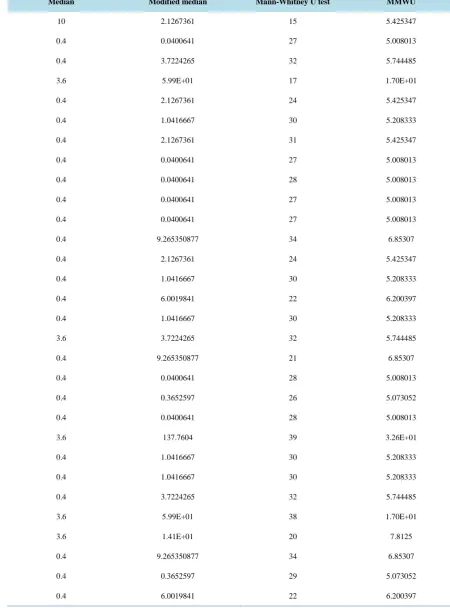
Table 5. Test statistic value of sample size 5.
Median Modified median Mann-Whitney U test MMWU
10 2.1267361 15 5.425347
0.4 0.0400641 27 5.008013
0.4 3.7224265 32 5.744485
3.6 5.99E+01 17 1.70E+01
0.4 2.1267361 24 5.425347
0.4 1.0416667 30 5.208333
0.4 2.1267361 31 5.425347
0.4 0.0400641 27 5.008013
0.4 0.0400641 28 5.008013
0.4 0.0400641 27 5.008013
0.4 0.0400641 27 5.008013
0.4 9.265350877 34 6.85307
0.4 2.1267361 24 5.425347
0.4 1.0416667 30 5.208333
0.4 6.0019841 22 6.200397
0.4 1.0416667 30 5.208333
3.6 3.7224265 32 5.744485
0.4 9.265350877 21 6.85307
0.4 0.0400641 28 5.008013
0.4 0.3652597 26 5.073052
0.4 0.0400641 28 5.008013
3.6 137.7604 39 3.26E+01
0.4 1.0416667 30 5.208333
0.4 1.0416667 30 5.208333
0.4 3.7224265 32 5.744485
3.6 5.99E+01 38 1.70E+01
3.6 1.41E+01 20 7.8125
0.4 9.265350877 34 6.85307
0.4 0.3652597 29 5.073052
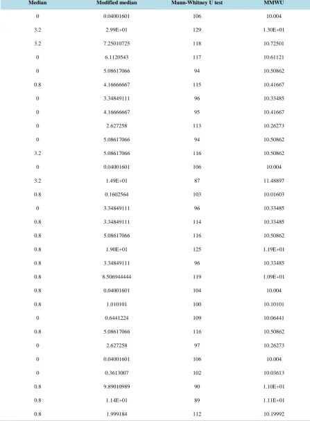
Table 6. Test statistic value of sample size 10.
Median Modified median Mann-Whitney U test MMWU
0 0.04001601 106 10.004
3.2 2.99E+01 129 1.30E+01
3.2 7.25010725 118 10.72501
0 6.1120543 117 10.61121
0 5.08617066 94 10.50862
0.8 4.16666667 115 10.41667
0 3.34849111 96 10.33485
0 4.16666667 95 10.41667
0 2.627258 113 10.26273
0 5.08617066 94 10.50862
3.2 5.08617066 116 10.50862
0 0.04001601 106 10.004
3.2 1.49E+01 87 11.48897
0.8 0.1602564 103 10.01603
0 3.34849111 96 10.33485
0.8 3.34849111 114 10.33485
0.8 5.08617066 116 10.50862
0.8 1.90E+01 125 1.19E+01
0.8 3.34849111 96 10.33485
0.8 8.506944444 119 1.09E+01
0.8 0.04001601 104 10.004
0.8 1.010101 100 10.10101
0 0.6441224 109 10.06441
0.8 5.08617066 116 10.50862
0 2.627258 97 10.26273
0 0.04001601 106 10.004
0 0.3613007 102 10.03613
0.8 9.89010989 90 1.10E+01
0.8 1.14E+01 89 1.11E+01
Table 7. Test statistic value of sample size 50.
Median Modified median Mann-Whitney U test MMWU
1.96 2.02E+01 2413 5.04E+01
0.04 2.4359713 2457 5.01E+01
0.36 0.77464 2547 5.00E+01
0.36 134.0615 2807 5.27E+01
0.04 3.10144281 2481 5.01E+01
0.36 3.10144281 2719 5.12E+01
1 7.86466359 2498 5.00E+01
0.04 0 2489 5.00E+01
3.24 6.24E+01 2720 5.12E+01
0.36 5.02769078 2469 5.01E+01
3.24 83.71228 2750 5.17E+01
0.36 3.18E+01 2385 5.06E+01
1 6.64E+01 2324 5.13E+01
1.96 3.96E+01 2681 5.08E+01
0.64 1.55E+01 2623 5.51E+01
7.84 2.65E+01 2906 5.51E+01
0.04 3.88E+01 2406 5.05E+01
0.36 0.05760133 2519 5.00E+01
0.36 9.03251706 2450 5.02E+01
0.04 5.39401309 2467 5.01E+01
0.04 0.2704292 2538 5.00E+01
3.24 124.258 2797 5.25E+01
3.24 149.5787 2822 5.30E+01
0.36 1.88E+01 2416.5 5.04E+01
0.04 8.555579317 2598 5.02E+01
0.36 2.99E+01 2661 5.06E+01
0.36 0.1024042 2517 5.00E+01
4.84 2.99E+01 2661 5.06E+01
1 1.4408299 2495 5.00E+01
Table 8. Test statistic value of sample size 100.
Median Modified median Mann-Whitney U test MMWU
0 2.23E+01 10286 100.2233
0.32 2.92E+01 10320 100.2925
0.72 5.18E+01 9691 100.5182
0.32 7.846151383 9910 100.0785
1.28 8.88829316 10199 100.0889
2 278.4764 9227 102.7848
5.12 193.564 9361 101.9356
1.28 5.39E+01 9684 100.5387
0 1.7959225 10117 100.018
0.08 5.38529858 9934 100.0539
0.32 4.32827258 9946 100.0433
0.08 2.2505064 10125 100.0225
1.28 0 10357 100.3784
0.32 3.765017 10147 100.0377
2.88 233.3302 9295 102.3333
1.28 2.65E+01 10307 100.2649
0 3.88E+01 9739 100.3884
0.32 1.2101464 10105 100.0121
0.32 4.7546596 10159 100.0475
1.28 104.7176 10559 101.0472
2 294.7239 9204 102.9472
0.72 8.301285418 10194 100.083
3.92 157.6999 9427 101.577
1.28 5.48E+01 10418.5 96.96971
0.32 4.24540158 9947 100.0425
0 5.29279989 10165 100.0529
0.08 5.29279989 9935 100.0529
0.08 4.24540158 9947 100.0425
0.08 2.90E+01 9781 100.2903
Table 9. Variances of the test statistic considered.
Type of distr. Test statistic 5 10 50 100
Symmetric distribution
Median 1.695 1.081 3.219 1.487
MMED 791.97 41.56 1748.91 7470.9
Asymmetric distribution
Median 2.072 0.924 1.575 1.918
MMED 82.56 64.37 3605.1 8664.9
Symmetric distribution
Mann-Whitney 27.513 124.97 22424.7 137572.1
MMWU 31.68 0.416 1.978 1.18
Asymmetric distribution
Mann-Whitney 25.082 125.18 23213.6 200042.0
MMWU 3.302 0.641 1.442 0.867
As shown in Table 10, M1 to M4 are the methods considered as M1 is the Median test and M2 is Modified Median test (MMED), M3 is the Mann-Whitney U test and M4 is Modified Mann-Whitney U (MMWU) test statistic.
All the ratios for the first and second rows are less than 1.0 which implies the method used as numerator is better and more reliable than the method used as denominator for all the sample sizes considered, i.e. Median Test is better than Modified Median intrinsically Adjusted for Ties (MMED) using Relative Efficiency (Table 11).
Moreover, considering methods 3 and 4 for asymmetric distribution, M4 (Modified Mann-Whitney U test) is better than M3 (Mann-Whitney U test) since the values of R.E are all greater than 1.0. Considering symmetric distribution, the efficiency of M3 (Mann-Whitney U test) is better/stronger for small sample size (5) and as sam-ple size increases, the strength of M4 (Modified Mann-Whitney U test) increases and outweighs M3 (Mann- Whitney U test); this implies that the method is inconsistent because its efficiency decreases as sample size in-creases.
As shown in Table 12, Median test has lower error rate which makes it better than MMED. This can be inter-preted thus, the usual Median test statistic is a better test statistic when testing relevant hypothesis. Error rate of MMED increases as sample size increases which implies MMED is better used for small sample sizes than the large sample size; but Median test statistic is found to be more adequate for both small and large sample sizes and hence should be preferable.
As shown in Table 13, Mann-Whitney U test statistic is more suitable irrespective of the nature of distribution of set of available data as the error rates of MMWU are significantly high. See Table 13. It can be deduced that the sensitivity of the test statistics is independent of sample size of the data but the distribution; either symmetric or asymmetric distribution.
Power of test were computed from Table 12 and Table 13.
Power of test is the sensitivity of a test statistic and the greater the value, the more sensitive the test statistic for both symmetric and asymmetric distributions. Median test is more sensitive than MMED because median has higher power than MMED irrespective of the sample sizes.
Considering both Mann-Whitney and MMWU, Mann-Whitney U test is more sensitivity than MMWU for both symmetric and asymmetric distribution. For better understanding of sensitivity of the four test statistics, line chart of power of test is constructed as shown in Figure 1 and Figure 2; Line chart can be used to show position of the strength or power of a test statistic especially in statistical inference. This shows test statistic with higher power with the maximum power of 1.0. See Figure 1 and Figure 2.
5. Graphical Illustration of Power of Test
As shown in Figure 1, irrespective of sample size; either large or small, the median test statistic has higher power than the modified median test which makes it more appropriate. The modified median test is sensitive to sample size as its power decreases as sample size increases.
Table 10. Relative efficiency of the test statistics.
Distribution 5 10 50 100
Asymmetric (M1M2) 0.0251 0.0144 0.0004 0.0002
Symmetric (M1M2) 0.0021 0.0260 0.0018 0.0002
Asymmetric (M3M4) 7.5960 195.2286 16098.1969 230728.9504
Symmetric (M3M4) 0.8685 300.4807 11337.0576 116586.5254
Table 11. Power of tests.
Type of distr. Test statistic 5 10 50 100
Symmetric distribution
Median 1 1 0.9667 0.9
MMED 0.6667 0.5 0.3333 0.1667
Asymmetric distribution
Median 1 1 0.9333 0.9
MMED 0.6667 0.6 0.2 0.1333
Symmetric distribution
Mann-Whitney 0.9 1 0.9333 0.9333
MMWU 0 0 0 0
Asymmetric distribution
Mann-Whitney 1 1 0.9667 0.9667
[image:14.595.85.539.109.521.2]MMWU 0 0 0 0
Table 12.Error rate of the median and modified median test statistics.
Type of distr. Test statistic 5 10 20 30 50 100
Symmetric distribution
Median 0.0000 0.0000 0.0000 0.0000 0.0333 0.1000
MMED 0.3333 0.5000 0.7000 0.8000 0.6667 0.8333
Asymmetric distribution
Median 0.0000 0.0000 0.0000 0.0000 0.0667 0.1000
MMED 0.3333 0.4000 0.6000 0.6667 0.8000 0.8667
Table 13. Error rate of Mann-Whitney and MMWU test statistics.
Type of distr. Test statistic 5 10 50 100
Symmetric distribution
Mann-Whitney 0.1000 0.0000 0.0667 0.0667
MMWU 1.0000 1.0000 1.0000 1.0000
Asymmetric distribution
Mann-Whitney 0.0000 0.0000 0.0333 0.0333
MMWU 1.0000 1.0000 1.0000 1.0000
Figure 1.Power of median and modified median test for both symmetric and asymmetric distribution.
0 0.2 0.4 0.6 0.8 1 1.2
5 10 50 100
Po
w
er
o
f T
es
t
Sample Sizes
[image:14.595.86.541.371.445.2] [image:14.595.86.492.446.699.2]Figure 2. Power of Mann-Whitney U and Modified Mann-Whitney U test for both
symme-tric and asymmesymme-tric distribution.
6. Summary and Conclusion
We have in this paper presented a nonparametric statistical method for the analysis of two sample tests. Based on the result of the analysis used, it is observed that for both symmetric and asymmetric distributions, median test is more efficient than Modified Median (MMED) test using relative efficiency as a measure of the efficiency of test statistic since the relative efficiency values are less than 1.0 while in terms of power of test for both symmetric and asymmetric distributions, median test is more sensitive than Modified Median (MMED) test since it has higher power. For Mann-Whitney U test and Modified Mann-Whitney U test (MMWU) using both relative efficiency and power of test, Mann-Whitney U test is more efficient and more sensitive than Modified Mann-Whitney U test (MMWU) since the relative efficiency values are greater than 1 and also it has higher power. In terms of sample size, efficiency of the method is independent of sample sizes except Modified Median Test which has higher power for small sample sizes.
References
[1] Gibbon, J.D. (1992) Nonparametric Statistics: An Introduction. Quantitative Applications in Social Sciences, Sage Publications, New York.
[2] Afuecheta, E.O., Oyeka, C.A., Ebuh, G.U. and Nnanatu, C.C. (2012) Modified Median Test Intrinsically Adjusted for Ties. Journal of Basic Physical Research, 3, 30-34.
[3] Mood, A.M. (1954) On the Asymptotic Efficiency of Certain Nonparametric Two-Sample Tests. Annals of Mathemat-ical Statistics, 25, 514-522. http://dx.doi.org/10.1214/aoms/1177728719
[4] Siegel, S. (1988) Nonparametric Statistics for the Sciences. McGraw-Hill, Kogakusha Ltd., Tokyo, 399.
[5] Mann, H.B. and Whitney, D.R. (1947) On a Test of Whether One of Two Random Variables Is Stochastically Larger than the Other. Annals of Mathematical Statistics, 18, 50-60. http://dx.doi.org/10.1214/aoms/1177730491
[6] Oyeka, I.C.A. and Okeh, U.M. (2013) Modified Intrinsically Ties Adjusted Mann-Whitney U Test. IOSR Journal of Mathematics, 7, 52-56. http://dx.doi.org/10.9790/5728-0745256
[7] Mumby, P.J. (2002) Statistical Power of Non-Parametric Tests: A Quick Guide for Designing Sampling Strategies. Marine Pollution Bulletin, 44, 85-87. http://www.elsevier.com/locate/marpolbul
http://dx.doi.org/10.1016/S0025-326X(01)00097-2
[8] Gupta, S.C. (2011) Fundamentals of Statistics. 6th Revised and Enlarged Edition, Himilaza Publishing House PVT Ltd., Mumbai, 16.28-16.31.
[9] Schaffer, M. (2010) Procedure for Monte Carlo Simulation. SGPE QM Lab 3, Monte Carlos Mark Version of 4.10.2010.
0 0.2 0.4 0.6 0.8 1 1.2
5 10 50 100
Po
w
er
o
f t
es
t
Sample sizes
[image:15.595.141.478.83.232.2]