A Nonparametric Test of Strategic Behavior in the Cournot Model

A Nonparametric Test of Strategic

Behavior in the Cournot Model

Deb, Rahul and Fenske, James

Yale University, Yale University

1 August 2009

Online at

https://mpra.ub.uni-muenchen.de/16560/

COURNOT MODEL

RAHUL DEB AND JAMES FENSKE†

Abstract. We devise a nonparametric test of strategic behavior in a multiproduct Cournot oligopoly. It is assumed that firms have cost functions that do not change over the period of observation but that market demand can change in each period. Market prices and firm-specific production quanti-ties are observed and it is assumed that neither the inverse demand functions nor the cost functions are known. The driving assumptions of the test are that market inverse demand functions are decreasing and differentiable at each period and that cost functions are increasing and convex for each firm. Under these very general conditions, we show that this test imposes strong restrictions on observed data. We apply the test to the crude oil market and find that strategic behavior is strongly rejected.

Keywords: Competitive behavior, Multiproduct Cournot oligopoly, Nonparametric test, Crude oil market, OPEC.

JEL Codes: C14, C72, D21, D43.

1. Introduction

The Cournot oligopoly is a canonical non-cooperative model in which firms individually choose what quantity of a homogenous good to produce and the price of the good is determined in the market. Tests for behavior of this type are difficult to implement, and often rely on parametric assumptions that are not robust to misspecification. This paper proposes a non-parametric test that overcomes this difficulty. This test is then applied to the world market for crude oil, in which nations choose their output of oil and the price is determined by international demand.

We say that a firm is behaving strategically if its production quantity is an optimal response to that of its competition. Formally, firmi is “strategic” if its choice of quantityqi satisfies

qi ∈argmax

q {

qP(q+Q−i)−Ci(q)}

where P(·) is the inverse demand function, Ci(·) is the cost function and Q−i is the aggregate

quantity produced by all the other firms in the market. Similarly, a subset of the firms in the

† _{Department of Economics, Yale University, 37 Hillhouse Ave, New Haven, CT 06511}

E-mail addresses: [email protected], [email protected].

Date: August 1, 2009.

We would like to thank John Quah for suggesting the problem and for providing helpful comments on an earlier draft. We would also like to thank Don Brown for suggestions which helped generalize the results. Needless to say, all errors are ours.

market are said to be strategic if the quantity produced by each one of them is a solution to the above maximization problem. If all the firms in the market are strategic then the market is in equilibrium. A trivial necessary condition for strategic behavior is that the first order condition of the above maximization problem is satisfied atqi. We use this first order condition to derive our

nonparametric test.

The data consists of market prices and firm-specific quantities. We do not observe firm profits or costs. Further, the market inverse demand function and the firms’ cost functions are not known to the researcher. Our test requires the following assumptions. We assume that the cost function of a given firm is convex, increasing and is the same over the period of observation. This assumption of a constant cost function is reasonable when the test is applied to observations spanning a short period of time. A change in the firm’s cost function might involve a change in its production technology or a restructuring of the organization of the firm. By contrast, we allow the market demand to change at each period of time. Demand is affected by fads, seasonality, advertising and numerous other factors, and it changes even over short periods of observation. We only assume that the market inverse demand function in each period is decreasing and differentiable.

A data set supports strategic behavior by a subset of firms M if it is possible to construct a cost function for each firm in M (which is invariant over the period of observation) and time specific market inverse demand functions such that, at each period of time, the observed quantity produced by each firm in M is an optimal response to the total quantity produced by every other firm in the market (where optimality is in terms of the constructed cost and inverse demand functions). We devise a nonparametric test of strategic behavior which consists of conditions that the data set must satisfy. As long as|M| ≥2, we show that in principle only two observations are required to reject strategic behavior. This is surprising given the generality of the model. It is not possible to test competitive behavior for a single firm nonparametrically as we can choose any arbitrary cost function and appropriately choose different inverse demand functions at each period of time which satisfy the firm’s first order condition.

As an application, we apply our test to price and quantity data from the crude oil market. There are two reasons for this choice of application. First, it is generally argued that there is some degree of collusion present in the market for oil. Since the test will reject strategic behavior in the presence of cooperation, demonstrating that it is capable of doing so in real data will show its usefulness. Second, certain members of the Organization of the Petroleum Exporting Countries (OPEC) and of the non-OPEC “fringe” have been argued not to behave collusively. This paper tests whether their behavior can be described as “strategic,” in the sense defined above.

2. Model

Consider a Cournot oligopoly with N firms. Each firm i chooses a quantity qi to produce where

1≤i≤N. We denote Q =q1+· · ·+qN as the total market quantity produced. Q−i =P_j6=iqj

refers to the total quantity produced by all firms except i. The market has an inverse demand functionP(Q) which depends on the total quantity produced. Assuming thatP depends only on

Qis the same as assuming that firms produce a homogenous good. Firmihas a cost function given by Ci(qi). The profit of firm iis given by

Πi(q1, . . . , qN) =qiP(Q)−Ci(qi).

The best response qi of firmitoQ−i is given by

qi∈argmax q

{qP(q+Q₋i)−Ci(q)}.

We make the following critical assumptions:

P(Q) is differentiable and decreasing inQ,

(PP)

Ci(qi) is increasing and convex in qi for all i.

(CC)

Assumption (PP) requires only that the demand curve be downward sloping and smooth, and assumption (CC) is a natural assumption for a cost function. These assumptions are extremely unrestrictive and as a result the model is very general.

Firms play the Cournot oligopoly game over T periods. We allow the inverse demand function to change over time and we denote the inverse demand in period t by Pt(·). At each t, Pt(·) is assumed to satisfy (PP). The firms’ cost functions are assumed to be constant over the period of observation. The observed data set D is a series of market prices and firm specific quantities observed overT periods or

D≡ {(pt, q₁t, . . . , q_Nt )}T_t=1,

where pt _{is the observed market price and q}t

i is the quantity produced by firm i in period t.

We assume that firm specific costs and profits are not observed. In practice, it is often difficult to observe these especially for firms that are not publicly listed. The model can be adapted to take this added information into account. Needless to say, the availability of more information strengthens the ability of the to reject the testable restrictions of the model. Our final assumption is that

(INT) q_it>0 for all i, t.

This ensures that for each firm the optimal quantity does not lie on the boundary.1 This assumption seems reasonable as is it unusual to find an operational firm that completely shuts down production for a short period of time.

1_{We actually only requireq}t

i>0 for subset of firmsi∈M which we are testing for strategic behavior. This assumption

Definition 2.1. We say that a subset of firms M ⊆N are strategic in data set D if we can find time specific inverse demand functionsPt(·) for 1≤t≤T and firm specific cost functionsCi(·) for

i∈M such that, for alli∈M and t:

Pt(·) satisfies (PP) and Ci(·) satisfies (CC), (C1)

qt_i ∈argmax

q

{qPt(q+Qt_−i)−Ci(q)}.

(C2)

In other words, the subset of firms are said to be strategic if they are best responding to the total quantity produced by all the other firms at each time period. If entire set of firmsN are strategic in the data set D, then D is said to support equilibrium. An inherent assumption in the above definition is that firms do not take into account future profits in current decisions. Hence, we are not testing for equilibrium of the repeated Cournot oligopoly. We should point out that since the equilibrium described by the above definition is a Nash equilibrium in each period, it is also an equilibrium of the repeated game. However, folk theorems tell us that repeated games have a much larger set of equilibria and given that we do not observe discount factors, there is no hope of being able to reject equilibrium in repeated Cournot oligopoly. We now derive the nonparametric test of the above model.

3. The Nonparametric Test

The test proposed in this section is connected to two strands of distinct literatures. Optimal behavior in the Cournot oligopoly model has been tested in the industrial organization literature. The survey of Geroski (1988) describes some of these tests and cites numerous others. Unlike the test proposed in this paper, they are parametric and often require additional data such as firm revenues, profits or market shares. The present paper is most closely related to the small literature that generalizes the insights of the revealed preference literature (see for example Varian (1982) and Varian (1984)) to game theoretic settings. In general, nonparametric tests of game theoretic models are difficult to design and implement, and moreover, they impose very weak or no restrictions on observed data (see Carvajal (2004), Deb (2008)). By contrast, the test in this paper is both intuitive and computationally efficient.

3.1. Strategic Behavior. We now state the nonparametric test of strategic behavior for M ⊆N

firms. The test consists of solving a system of|M|T2 linear inequalities with|M|T+T unknowns. If a firm is behaving strategically, these inequalities can be shown to be necessary as they follow from the first order conditions. The proof in the appendix shows them to be sufficient as well.

Proposition 3.1. We are given an observed data set D≡ {(pt, q₁t, . . . , q_Nt )}T_t=1 satisfying (INT). A subset M ⊆ N of firms are strategic on D, if and only if, the following system of inequalities have positive solutions for unknown constants C_it, λt

C_it′ ≥C_it+ (pt−λtq_it)(q_it′ −q_it),

(1)

pt_−λt_qt i >0

for all i∈M, t, t′.

Before we discuss the properties of the test, we would like to present an example of theoretical data that violates the inequalities above. This shows immediately that the above test is not vacuously satisfied on all data sets. This example also captures the power of the test. As stated above, game theoretic models in general are hard to test nonparametrically due to the presence of externalities. Moreover, our model allows for changing market demand at each period. It is thus surprising that we can reject competitive behavior with only two observations.

Example 3.1. Consider data setD={(p1, q1₁, q₂1),(p2, q2₁, q2₂)} consisting of two observations and two firms. We test to see if both firms are strategic, which in this two-firm would correspond to an equilibrium. Observed prices and quantities are

At t= 1 : p1 = 1, q₁1= 2, q1₂ = 1,

At t= 2 : p2 = 2, q₁2= 1, q2₂ = 4.

Since 0< λt< p_qtt i

for all i, t, we can infer that

0< λ1< 1

2 and 0< λ

2 _< 1

2

We now check to see if we can satisfy the cost inequalities of the first firm. The above implies

C₁1≥C₁2+ (p2−λ2q₁2)(q1₁−q2₁)

=⇒C₁1−C₁2 ≥2−λ2 > 3

2 and

C₁2≥C₁1+ (p1−λ1q₁1)(q2₁−q1₁) =⇒C₁1−C₁2 ≤1−2λ1 <1.

Since the above inequalities cannot be satisfied simultaneously, the observed data cannot correspond to an equilibrium.

A curious aspect of Proposition 3.1 is highlighted by the above example. It is precisely the presence of the second firm that helps bound λ2, which in turn precludes the inequalities from having a solution. When there is only a single firm (monopolist) in the market, any data can be rationalized. In this model, the presence of the externality actually strengthens its testable implications. This goes against standard intuition. The reason for this is that the only thing that matters to a firm is the total quantity produced by all the other firms. Hence, the larger the setM, the more likely we can reject strategic behavior as it is more likely to find a single firm that is not best responding, This is sufficient for the test to reject. This in turn implies that if strategic behavior for a subset

M of firms cannot be supported then we cannot support strategic behavior for any M′ ⊇M.

Finally, it is also worth pointing out that the inequalities in Proposition 3.1 are linear in the unknowns. This means that the test involves checking that a linear programme has a feasible solution. Linear programming is computationally inexpensive and this makes our test practical as is highlighted by the empirical section.

3.2. Collusion. It is possible to use the test to check for collusive behavior. Consider the case of 3 firms {1,2,3} engaged in a Cournot oligopoly. If we run the test on the set M = {1,2} and the test is rejected, we can conclude that the data does not support individually strategic behavior for firms 1 and 2. We can treat firm 1 and 2 as a single firm, that is, we sum the quantities they produce and we can test this combined firm along with firm 3 for strategic behavior. If the test is not rejected, then the data supports collusive behavior for firms 1 and 2.

Our test is robust to combining firms, because all the necessary assumptions are satisfied on the combined firm. If the cost of production for a set of colluding firmsO⊆N is increasing and convex, then we are free to treat them as a single entity. The following lemma states this formally. The proof is trivial and is omitted.

Lemma 3.1. If cost functions Ci(qi) for individual firms i ∈ O are increasing and convex, then

the cost function for the combined firm given by

CO(q) = min

{qi:i∈O}

X

i∈O

Ci(qi)

such that

X

i∈O

qi =q

is increasing and convex in q.

The following section shows that the test can be generalized to a multiproduct setting.

4. Multiproduct Oligopoly

of the different goods (see for example Brander and Eaton (1984) and Bulow et al. (1985)). There are K markets indexed by 1 ≤ k ≤ K. There is an inverse demand function Pk(Q1, . . . , Qk)

corresponding to each market k. The price in market k can depend on the total quantities of the goods produced in other markets as well. This allows us to test for strategic behavior in market in which goods are substitutes.

Firms can be active in the entire market or on a subset of the market. In reality, firms that manufacture a variety of different products often compete with firms that operate in fewer markets or with firms that specialize in a single product. We use Ki ⊆ {1, . . . , K} to denote the set of

markets where firm i competes. Each firm now produces a |Ki|dimensional vector of quantities,

once again denoted by qi. We use the added subscript in qik to denote the quantity of good k

produced by oligopolistiwhen k∈Ki. The cost functionCi(qi) of an oligopolistidepends on the

entire |Ki|dimensional vector of quantities produced, where

Ci :R|Ki|→R.

This models the potential synergies in production. The total quantity in marketk is just the sum of quantities produced by firms active in that market or

Qk=

X

{i:k∈Ki}

qik.

Q₋ik is the sum of quantities of all active firms in market kbarring i. Profits are given by

Πi(q1, . . . , qN) =

X

k∈Ki

qikPk(Q1, . . . , QK)−Ci(qi)

and best responses are a vector of quantities given by

qi∈argmax q

{X

k∈Ki

qkPk(q1+Q−i1, . . . , qk+Q−ik, . . . , qK+Q−iK)−Ci(q)}.

We make the following assumptions about the cost functions and inverse demand functions which are analogous to the single product case.

Pk(Q1, . . . , QK) is differentiable,

∂Pk(Q1, . . . , QK)

∂Qk

<0 and ∂Pk(Q1, . . . , QK)

∂Ql

≤0 for alll6=k,

(PP’)

Ci(qi) is increasing inqik for all k∈Ki and convex in qi for all i.

(CC’)

Assumption (PP’) implies that the price in marketk must be decreasing in the quantity of goodk

produced and nonincreasing in the quantity of all other goods. In particular, if ∂Pk(Q1,...,QK)

∂Ql = 0

for alll6=k, this implies that the price of goodkisn’t affected by the quantities of the other goods produced or in other words, there is no substitute for goodk in the market.

Once again, firms compete overT periods. The inverse demand function can change over time but the firms’ cost functions are assumed to be constant. The observed data setDis a series of market prices and firm specific quantities orD≡ {(pt_{, q}t

areK dimensional vectors

pt= (pt₁, . . . , pt_K),

and the quantity qt

i is a |Ki| dimensional vector. As in the single product case, we make the

assumption that quantities lie in the interior. Formally,

(INT’) q_ikt >0 for all k∈Ki, for alli, t.

The assumption only requires firms to be producing positive quantities in markets in which they are active. Strategic behavior is analogously defined and involves constructing a cost function for each firm and an inverse demand function for each good at each time period. We now state our test for the multiproduct oligopoly. The proof uses the same argument as the proof of Proposition 3.1 and is in the appendix.

Proposition 4.1. We are given an observed data set D≡ {(pt_{, q}t

1, . . . , qNt )}Tt=1 satisfying (INT’).

A subsetM ⊆N of firms are strategic onD, if and only if, the following system of inequalities have positive solutions for unknown constantsC_it′ and nonnegative solutions for unknownK2 dimensional vectors λt= (λt₁, . . . , λt_K) where λt_k= (λt_k1, . . . , λt_kK)

C_it′ ≥C_it+P

k∈Ki(p

t

k−

P

l∈Kiλ

t lkqtil)(qt

′

ik−qikt ),

(3)

pt_k−P

l∈Kiλ

t

lkqilt >0 if k∈Ki

(4)

λt_kk >0 (5)

for all i∈M, k, t, t′.

Like the single product case the constantsλt_lk=−∂P

t l

∂Qk(Q

t

1, . . . , QtK) represent the marginal decrease

in the price in marketl by an additional unit produced in marketk. The additional inequality (5) ensures prices in marketkare decreasing in quantity of goodkproduced. Since we also requireλlkto

be nonnegative, we can ensure that an inverse demand function satisfying (PP’) can be constructed. We end this section with the obvious generalization of Example 3.1 to the multiproduct setting. This example considers the case of two competing firms in two markets and it captures the full generality of our results.

Example 4.1. Consider data set D = {(p1, q1₁, q₂1),(p2, q2₁, q₂2)} consisting of two observations of two firms competing in two markets (K = 2). We assume that both firms are active in both markets or

K1=K2={1,2}.

We consider M = {1,2}. That is we are testing for equilibrium. Observed prices and quantities are

Att= 1 : p1₁=p1₂= 1 q₁₁1 =q₁₂1 = 2 q₂₁1 =q1₂₂= 1 Att= 2 : p2₁=p2₂= 2 q₁₁2 =q₁₂2 = 1 q₂₁2 =q2₂₂= 4

Proposition 4.1 implies that pt_k−P

l∈Kiλ

t

klqtik > 0 if k ∈ Ki for all i, k and that λtkl ≥0 we can

infer that

0< λ1₁₁+λ1₂₁< 1

2, 0< λ

1

12+λ122<

0< λ2₁₁+λ2₂₁< 1

2, 0< λ

2

12+λ222<

1 2

We now check to see if we can satisfy the cost inequalities of the first firm. The above implies

C₁1 ≥C₁2+ [p2₁−λ2₁₁q₁₁2 −λ2₂₁q₁₂2 ][q1₁₁−q2₁₁] + [p2₂−λ2₁₂q2₁₁−λ2₂₂q2₁₂][q₁₂1 −q₁₂2 ] =⇒C₁1−C₁2 ≥4−(λ2₁₁+λ2₂₁)−(λ2₁₂+λ2₂₂)>3

and

C₁2 ≥C₁1+ [p1₁−λ1₁₁q₁₁1 −λ1₂₁q₁₂1 ][q2₁₁−q1₁₁] + [p1₂−λ1₁₂q1₁₁−λ1₂₂q1₁₂][q₁₂2 −q₁₂1 ] =⇒C₁1−C₁2 ≤2−2(λ1₁₁+λ1₂₁)−2(λ1₁₂+λ1₂₂)<2

Since the above inequalities cannot be satisfied simultaneously, the observed data cannot correspond to an equilibrium.

5. Application: The World Market for Crude Oil

5.1. Background and Literature. Petroleum accounts for more than one third of global energy consumption, and in April 2009 world oil production was more than 72 million barrels per day (Monthly Energy Review (MER), 2009). Accounting for roughly one third of global oil production, the OPEC is a dominant player in the international oil market. OPEC was founded in 1960 and exists, in its own words, “to co-ordinate and unify petroleum policies among Member Countries, in order to secure fair and stable prices for petroleum producers; an efficient, economic and regular supply of petroleum to consuming nations; and a fair return on capital to those investing in the industry.” OPEC rose to prominence during the energy crises of the 1970s for its embargo in response to Western support of Israel during the 1973 Yom Kippur War. Since the start of the 1980s, with the abolition of US price controls and increased production by the rest of the world, OPEC’s influence on oil prices has declined. Beginning in 1982, OPEC began to allocate production quotas to its members, replacing a system of posted prices. This has not, however, permitted OPEC to dictate world prices, since the majority the world’s oil is produced by non-members and the only sanction available to police its members is Saudi Arabia’s spare capacity.

OPEC’s stated aims are effectively those of a cartel, but its ability to set world oil prices is question-able; hence, a large literature has emerged that attempts to model its actions and to test whether these models fit its observed behavior. No consensus has emerged. Smith (2005) argues that many of the statistical tests implemented have low power across alternative hypotheses, and that many of these look for the presence of behavior that could be consistent with either cooperation or collu-sion. Gault et al. (1999), for example, are unable to distinguish between alternative models of the allocation of quotas within OPEC.

conversely, he cannot reject the competitive model. Jones (1990) and Ramcharran (2002) find supporting results for the periods from 1983 to 1988 and 1973 to 1997, respectively. G¨ulen (1996), similarly, finds that OPEC production influenced prices from 1982 to 1993, though it did not have to restrain output to benefit from high prices during the 1970s. Loderer (1985), by contrast, finds that the outcomes of OPEC meetings had little to no effect on oil prices from 1974 to 1980, before the quota system was adopted, but did affect prices from 1981 to 1983.

For the most part, the literature has suggests that OPEC is a “weakly functioning cartel” of some sort, and is not “competitive” in either the price-taking or non-cooperative Cournot senses. Griffin and Neilson (1994) argue that OPEC followed a swing producer strategy from 1983 to 1985, when Saudi Arabia’s profits fell below Cournot levels and that country began to adopt a tit-for-tat strategy. Using co-integration tests, Dahl and Y¨ucel (1991), do not find evidence that either the OPEC or the non-OPEC “fringe” behave competitively, suggesting that OPEC is best described by loose coordination. Alhajji and Huettner (2000) find no statistical support for Cournot or competitive models of the world oil market, and are only unable to reject a model in which Saudi Arabia plays the role of dominant producer. Spilimbergo (2001) estimates Euler equations for each country; he rejects the model of a market-sharing cartel for Saudi Arabia, while finding that Iraq and Nigeria constitute a revenue-maximizing “expansionist fringe” that regularly cheats on its quotas. Smith (2005) finds that OPEC members compensate for output fluctuations of other countries much less than do non-OPEC countries, suggesting a rejection of the competitive, Cournot, Stackelberg, Bertrand, and frictionless cartel models in favor of a cartel model with frictions. Almoguera and Herrera (2007) find that OPEC has switched between competitive and collusive behavior over its history, while on average its actions are best described by Cournot competition with the non-OPEC countries as a competitive fringe.

Together, these results suggest that the hypothesis of pure Cournot behavior should be rejected by our nonparametric test. Applying the test to the world oil market will demonstrate that, although the test is very general, it can reject the restrictions of Cournot competition in real world data. Further, the tests of alternative models of OPEC behavior that have been made suffer from two shortcomings that are overcome in the present paper. First, many of these tests rely on parametric assumptions about the functional forms taken by market demand, countries’ objective functions and production costs. Second, several of these tests require that factors shifting the cost and inverse demand functions be observed, and rely on constructed proxies such as estimates of countries’ extraction costs, the presence of US price controls, and involvement of an OPEC member in a war. The non-parametric test implemented in the current paper only needs output and quantity to be implemented.

China, Egypt, Mexico, Norway, the United States, and the United Kingdom).2 This series also contains total world output. The data are available from January 1973 until April 2009, giving a total length of T = 436 months and ¯M ×T = 8248 country-month observations. There are only seven instances in the data in which an individual country’s monthly production is zero,3 and so false acceptances and rejections of the test due to violation of this assumption will be small in number. The second source of data is a series of oil prices published by the St. Louis Federal Reserve, in dollars per barrel. This series is deflated by the monthly consumer price index reported by the Bureau of Labor Statistics, so that prices are in 2009 US dollars. Since the time windows over which Cournot behavior is tested are short (twelve months or less), the adjustment for inflation should not matter to the results.4

Each test consists of using a linear programming algorithm to find whether there exist Ct

i and

λt that satisfy the inequalities in Proposition 3.1 for M countries during a window of time of length W. If these exist, this subset of the data can be rationalized within the Cournot model, i.e. strategic behavior by theseM countries is supported by the data during the period tested. If, instead, the data cannot be rationalized, it is not consistent with the strategic behavior. As will be shown below, as M and W increase, it is more likely that at least one country is not behaving strategically in at least one period, and so it is more likely that it will not be possible to satisfy the set of inequalities. Rather than performing a single test for whether the entire data series can be rationalized, we select a number of firms M, and then test whether the subsets data for each of the M_M¯

possible combinations of firms in each of the T + 1−W periods of length W can be rationalized. We then report the percentage of these M_M¯

×(T + 1−W) cases in which strategic behavior is rejected. The time windows selected are short; W is either 3 months, 6 months, or 12 months. This is in keeping with the assumption that cost functions do not change over the period of the test. If a test is able to reject for a small amount of data (for example, three countries over three months), it demonstrates that, despite the generality of the non-parametric framework, the test has considerable power to detect non-strategic behavior in real data.

5.3. Results. Table 1 presents the percentage of cases for which Cournot behavior could not be rationalized by subsets of the data over groups of 2, 3, 6 and 12 OPEC countries within windows of 3, 6, and 12 months. The results are surprisingly consistent – once there are more than a handful of observations used, the behavior of OPEC members cannot be explained by the Cournot model. For nearly 90% of six-month periods with three countries, the test rejects strategic behavior. Once six countries are included, fewer than one six-month case in ten thousand can be rationalized. The test, then, has surprising power to reject strategic behavior when applied to real data. For the

2_{Russia and the former Soviet Union are not used here, because the two are not comparable units. Although the}

composition of OPEC has changed over the course of the data (Ecuador left in 1994 and returned in 2007, Gabon left in 1995, Angola joined in 2007, and Indonesia left in 2007), the overall pattern of rejecting Cournot behavior below does not depend on what countries are considered to be part of OPEC. Reported tests consider groups of 2, 3, 6, and 12 member states; these overwhelmingly reject Cournot behavior for almost all country groups in periods longer than a few months.

Table 1. Rejection Rates: OPEC

Number of Countries

2 3 6 12

Window

3 Months 0.28 0.54 0.89 1.00

6 Months 0.65 0.89 1.00 1.00

12 Months 0.90 0.99 1.00 1.00

Notes:_{The rejection rate reported is the proportion of cases that were rejected. For example, there are 436 + 1}−3 =

434 three month periods in the data. There are 66 possible combinations of two out of twelve OPEC members. The entry for two countries and three months, then, reports that out of the 434×_{66 = 28,644 possible tests of two opec}

members over three months, 8138, or 28% could not be rationalized.

behavior of OPEC members, the conclusions are stark. If there is a model to describe OPEC, Cournot oligopoly is not it. Specifically, one of two conditions are warranted. First, if it is true that countries produce their output simultaneously and the world price is set by the intersection of inverse demand with total world output, then OPEC members are clearly not behaving according to their optimal non-cooperative strategies. Second, it may be that the basic assumptions of the Cournot model – simultaneous production, a single market inverse demand function, and stable convex costs – do not hold.

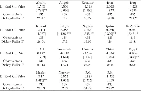
If countries are not producing according to their optimal non-cooperative strategies, two possible alternatives are collusion and price-taking. Some evidence against the latter is presented in Table 2. If countries are behaving as price takers, they should produce to where price equals marginal cost, and so increases in the world price of oil should be associated with increases in output. This table presents regression results for each countryiof the form:

(6) ∆qit=β0+β1∆pit+ǫit.

The table reports the estimates of β1, along with Dickey-Fuller tests for a unit root in the ∆qit

series. In all cases, the null of a unit root is rejected, consistent with stationarity of the ∆qit series.

For the ∆pit series, the associated test statistic is 13.99, which is also consistent with stationarity.

For most of the countries in the data, there is no positive correlation of output with prices, and so price-taking behavior can be rejected. Though a marginally significant correlation is found for Saudi Arabia, the conclusion that it is a price-taker is a priori unreasonable. For four OPEC members (Algeria, Libya, Nigeria, Qatar), there is a positive correlation of output with the world price, and so price-taking cannot be ruled out for this group. The lack of such a result for the majority of OPEC members suggests, however, the deviation from individualistic Cournot behavior is towards collusion, rather than towards perfect competition.

Table 2. Correlations of ∆qit with ∆pit

Algeria Angola Ecuador Iran Iraq

D. Real Oil Price 1.563 0.516 -0.145 2.098 -0.323

[0.732]** [0.636] [0.199] [1.873] [5.925]

Observations 435 435 435 435 435

Dickey-Fuller F 22.47 17.9 25.27 19.18 21.02

Kuwait Libya Nigeria Qatar S. Arabia

D. Real Oil Price -2.411 3.288 3.263 0.976 9.661

[4.057] [1.126]*** [1.645]** [0.399]** [5.461]*

Observations 435 435 435 435 435

Dickey-Fuller F 26.54 17.3 19.66 28 21.81

U.A.E. Venezuela Canada China Egypt

D. Real Oil Price 0.177 -0.962 -0.924 -1.257 0.784

[1.789] [1.624] [1.040] [1.294] [0.338]**

Observations 435 435 435 435 435

Dickey-Fuller F 21.13 17.74 26.93 26.8 22.37

Mexico Norway U.S. U.K.

D. Real Oil Price 3.17 0.575 -1.935 -1.726

[1.470]** [1.633] [3.725] [1.465]

Observations 435 435 435 435

Dickey-Fuller F 25.33 32.82 24.72 23.92

***Significant at 1%, **Significant at 5%, *Significant at 10%.

Notes: _{Robust standard errors in brackets. All regressions also include a constant. Dickey-Fuller tests are for the}

∆qi, where the 10% critical value with 434 observations is 2.570.

would have these countries taking into account their own impacts on the world price when choosing output. Table 3, then, repeats the analysis of Table 1 for the sample of 7 non-OPEC countries. Here, however, the results are again strongly against the Cournot model. For almost all six month periods, when at least three countries are considered, the data cannot be rationalized by the Cournot model. While the results in Table 2 are consistent with Egypt and Mexico behaving as price takers, this is not the case for Canada, China, Egypt, Norway, the U.S., or the U.K. Again, either the underlying presumptions of simultaneous production, convex cost functions that are stable over the course of the test, and a world inverse demand curve are incorrect, or oil production by even non-OPEC countries is not well described by their optimal strategies in the Cournot game.

Table 3. Rejection Rates: Non-OPEC

Number of Countries

2 3 7

Window

3 Months 0.44 0.75 0.75

6 Months 0.83 0.98 0.98

12 Months 0.96 1.00 1.00

Finally, it is interesting to test whether particular pairs of countries are behaving according to their non-cooperative optimums. Table 4 then presents results for four country pairs – Qatar and Ecuador (the smallest OPEC members by output), Egypt and Norway (the smallest non-OPEC members by output), Iraq and Kuwait, and Iraq and Nigeria, the latter pairs having reputations as part of the quota-violating “expansionist fringe.” Even for these sets of countries the data are not able to rationalize their output decisions for most six-month periods and can only do so for a small percentage of twelve-month periods. For Iraq and Kuwait, many of the periods during which strategic behavior could not be rejected overlap with their brief periods of zero production, suggesting these rejections are spurious. Even for these pairs of countries, optimal response in the Cournot game cannot explain their behavior for most of the period from 1973 to 2009.

Table 4. Rejection Rates: Other Cases

Country Pairs

Qatar/Ecuador Egypt/Norway Iraq/Kuwait Iraq/Nigeria

Window

3 Months 0.37 0.43 0.37 0.38

6 Months 0.77 0.83 0.72 0.74

12 Months 0.96 0.97 0.93 0.95

Notes:_{Rates report the percentage of intervals during which behavior of the two countries could not be rationalized.}

6. Conclusion

This paper has introduced a nonparametric test for strategic behavior in a Cournot oligopoly. It has extended this test to cover a multi-product case with synergies in production and substitutability between goods in the market. It has applied the test to the world market for oil, and found that neither production by OPEC members nor by the non-OPEC fringe, even over short periods, can be explained using the Cournot model with stable, convex cost functions.

Appendix A. Proof Of Proposition 3.1

The proof of our main result turns on the following simple lemma. This lemma is inspired by the work of Chavas and Cox (1993) and Forges and Minelli (2009) who study consumption over nonlinear budget sets.

Lemma A.1. Let f be a concave differentiable function and let g be a concave function. Then

x∗ ∈argmax_x{f(x) +g(x)}

if, and only if,

x∗∈argmaxx{f(x∗) +f′(x∗)(x−x∗) +g(x)} .

while the Cournot oligopoly with linear costs is a common example of a Potential game (Monderer and Shapley (1996)), the general Cournot oligopoly game studied in this paper is not a Potential game. This precludes using arguments which specifically use properties of Potential games (see Deb (2009)).

Proof. Necessity:

Consider an arbitrary firm i. Assumption (INT) ensures that the first order condition is satisfied at the observed data points because they constitute an equilibrium. Formally,

C_i′(q_it) =pt+dP

t

dQ(Q

t_)qt i >0

whereC_i′(qt

i) is the subgradient ofCi(·) atqit. Moreover since Ci is convex the following inequality

must hold

Ci(qt

′

)≥Ci(qit) +Ci′(qit)(qt

′

i −qit).

Setting C_it=Ci(qit) andλt=−dP

t

dQ(Q

t_{) we can satisfy inequality (1). Since C}

i(·) is increasing we

can satisfy the inequality (2) as well.

Sufficiency:

We start off by defining cost functionCi(·) as the upper envelope of the right side of the inequalities.

Formally

Ci(q) = max

1≤t≤T{C t

i + (pt−λtqit)(q−qit)}.

This function is clearly convex as it is the maximum of linear functions. Moreover

Ci(qit) = max

1≤s≤T{C s

i + (ps−λsqsi)(qit−qis)}

=C_it′+ (pt′−λt′q_it′)(qt_i−qt_i′) [where t′ is the argmax of the above]

≥C_it+ (pt−λtqt_i)(qt_i−qt_i) =C_it

If the inequality above is strict then we get a violation of the first inequality of (2) in the theorem. Hence Ci(q_it) =C_it. Moreover since pt−λtq_it>0,Ci is increasing.

We can always choose an arbitrary decreasing, strictly concave, smooth inverse demand function

Pt_{(·) such that P}t_(Qt_{) = p}t _and dPt

dQ(Qt) = −λt for each time period t. We now show that we

can rationalize the data using the derived functionsCi(·) and any inverse demand functions Pt(·)

chosen as above. Using Lemma A.1, we conclude that solving

max

q {qP

t_(q+Qt

−i)−Ci(q)},

for firm iis equivalent to solving the linearized problem

max

q

ptq_it+

pt+q_itdP

t_(Qt₎

dQ

(q−qt_i)−Ci(q)

where dP t

(Qt

)

dQ =−λ

t_{. Consider the latter problem. For any choice q}

i 6=qit, the maximand is given

by

ptq_it+ [pt−λtqt_i][qi−qit]−Ci(qi)

≤ptqi−λtqit(qi−qti)−Cit−[pt−λtqit](qi−qit)

=ptq_it−C_it

But an oligopolist can always guarantee herselfptqt_i−C_itin the linearized problem by producingqt_i. Hence, q_it maximizes the linearized problem and is hence a best response to Qt_−i at the observed data points. The same argument applies for the other firms and this completes the proof.

Appendix B. Proof Of Proposition 4.1

Lemma A.1 generalizes in the obvious way to functions defined on vectors.

Proof. Necessity:

Consider an arbitrary firm i. Assumption (INT’) ensures that the first order condition is satisfied at the observed data points because they constitute an equilibrium. Formally

∇kCi(qit) =ptk+

X

l∈Ki

∂Pt l

∂Qk

(Qt₁, . . . , Qt_K)q_ilt >0

where∇kCi(qit) is the kth component of the subgradient∇Ci(qit) of Ci(·) at qit. Moreover since Ci

is convex the following inequality must hold

Ci(qt

′

i )≥Ci(qit) +∇Ci(qit).(qt

′

i −qit).

Setting C_it=Ci(qit) andλtlk =− ∂Pt

l

∂Qk(Q

t

1, . . . , QtK) we can satisfy the inequality (3). Since Ci(·) is

increasing we can satisfy the second inequality (4) as well.

Sufficiency:

We start off by defining cost functionCi(·) as the upper envelope of the right side of the inequalities.

Formally

Ci(q) = max

1≤t≤T{C t

i +

X

k∈Ki

(pt_k− X

l∈Ki

λt_lkqt_ik)(qk−qtik)}.

This function is clearly convex as it is the maximum of linear functions. Moreover

Ci(qit) = max

1≤s≤T{C s

i +

X

k∈Ki

(ps_k−X

l∈Ki

λs_lkq_iks)(q_ikt −qs_ik)}

=C_it′+ X

k∈Ki

(pt_k′−X

l∈Ki

λt_lk′q_ikt′)(q_ikt −qt_ik′) [where t′ is the argmax of the above]

≥C_it+ X

k∈Ki

(pt_k− X

l∈Ki

λt_lkqt_ik)(qt_ik−q_ikt )

If the inequality above is strict then we get a violation of the first inequality (3) in the proposition. Hence Ci(q_it) =C_it. Moreover since pt_k−P_l∈Kiλ

t

lkqikt >0,Ci is increasing.

We can always choose an arbitrary decreasing, strictly concave, smooth inverse demand function

Pt

k(·) such thatPkt(Qt1, . . . , QtK) =ptk and dPt

l

dQk(Q

t

1, . . . , QtK) =−λtlkfor each time periodtand each

k. We now show that we can rationalize the data using the derived functionsCi(·) and any inverse

demand functionsP_kt(·) chosen as above. we have shown that solving

max

q {

X

k∈Ki

qkPkt(q1+Qt−i1, . . . , qk+Qt−ik, . . . , qK+Qt−iK)−Ci(q)},

for firm iis equivalent to solving the linearized problem

max q    X

k∈Ki



pt_kq_ikt +  pt_k+

X

l∈Ki

q_ilt∂P

t

l(Qt1, . . . , QtK)

∂Qk



 q_k−qt_ik



−Ci(q)

   , where ∂P t l(Q

t

1,...,Q

t K)

∂Qk =−λ

t

lk. Consider the latter problem. For any choice qi 6=qit, the maximand is

given by

X

k∈Ki



pt_kqt_ik+  pt_k−

X

l∈Ki

qt_ilλt_lk



 qik−qikt



−Ci(qi)

≤ X

k∈Ki



pt_kq_ik−  

X

l∈Ki

qt_ilλt_lk



 q_ik−q_ikt



−C_it− X

k∈Ki

(pt_k− X

l∈Ki

λt_lkqt_ik)(q_ikt −q_ikt )

= X

k∈Ki

pt_kqt_ik−C_it

But an oligopolist can always guarantee herself P

k∈Kip

t

kqtik −Cit in the linearized problem by

producing qt_i. Hence, q_it maximizes the linearized problem and is hence a best response to Qt_−i at the observed data points. The same argument applies for the other firms and this completes the

proof.

References

[1] Almoguera, P. and Herrera, A. (2007), Testing for the cartel in OPEC: noncooperative collusion or just noncooperative?.Working Paper.

[2] Alhajji, A. and Huettner, D. (2000), OPEC and World Crude Oil Markets from 1973 to 1994: Cartel, Oligopoly, or Competitive? The Energy Journal, 21(3), 31-60.

[3] Brander, J. and Eaton, J. (1984), Product Line Rivalry.American Economic Review, 74, 323-334.

[4] Bulow, J., Geanakoplos, J. and Klemperer, P. (1985), Strategic Substitutes and Complements. Journal of Political Economy, 93, 488-511.

[5] Carvajal, A. (2004), Testable Restrictions of Nash Equilibrium in Games with Continuous Domains.Working Paper.

[6] Chavas, J. P. and Cox, T. L. (1993), On Generalized Revealed Preference Analysis.The Quarterly Journal of Economics, 108(2), 493-506.

[8] Deb, R. (2008), Interdependent Preferences, Potential Games and Household Consumption.Working Paper. [9] Deb, R. (2009), A Testable Model Of Consumption With Externalities. Journal of Economic Theory, 144,

1804-1816.

[10] Forges, F. and Minelli, E. (2009), Afriats Theorem for General Budget Sets. Journal of Economic Theory, 144, 135-145.

[11] Gault, J., Spierer, J., Bertholet, J.and Karbassioun (1999), How does OPEC allocate quotas? Journal of Energy Finance and Development, 4(2), 137-148.

[12] Geroski, P. A. (1988), In Pursuit of Monopoly Power: Recent Quantitative Work in Industrial Economics.

Journal of Applied Econometrics, 3(2), 107-123.

[13] Griffin, J. (1985), OPEC Behavior: A Test of Alternative Hypotheses. The American Economic Review, 75(5), 954-963.

[14] Griffin, J. and Neilson, W. (1994), The 1985-86 oil price collapse and afterwards: what does game theory add? Economic Inquiry, 32(4), 543-561.

[15] G¨ulen, G. (1996), Is OPEC a cartel? Evidence from cointegration and causality tests. The Energy Journal, 17(2), 43-58.

[16] Jones, C. (1990), OPEC behaviour under falling prices: Implications for cartel stability.The Energy Journal, 11(3), 117-134.

[17] Monderer, D., and Shapley, L. (1996), Potential Games.Games and Economic Behavior, 14, 124-143. [18] Loderer, C. (1985), A Test of the OPEC Cartel Hypothesis: 1974-1983. The Journal of Finance, 40(3),

991-1006.

[19] Ramcharran, H. (2002), Oil production responses to price changes: an empirical application of the competitive model to OPEC and non-OPEC countries.Energy Economics, 24(2), 97-106.

[20] Spilimbergo, A. (2001), Testing the hypothesis of collusive behavior among OPEC members. Energy Eco-nomics, 23(3), 339-353.