Munich Personal RePEc Archive
How are social ties formed? : Interaction
of neighborhood and individual
immobility
Yamamura, Eiji
26 June 2010
Online at
https://mpra.ub.uni-muenchen.de/23543/
0
How are social ties formed? Interaction of neighborhood
and individual immobility.
Abstract
Using individual data from Japan, this paper investigates how a neighbor’s
immobility is associated with individual investment in social capital. It is found that
local homeownership has a positive effect on individual investment and that this effect
for individual homeowners is about 2.5 times larger than for renters.
Keywords: Social ties, Social capital, homeownership, length of residence.
1 1. Introduction
Since the seminal work of Putnam (2000), social capital has been regarded as an
influential social science concept, with the formation of social capital being a major
issue for researchers. From an economics viewpoint, it is critical to analyze what gives
individuals an incentive to invest in social capital (Glaeser et al. 2002). For instance,
empirical works explore how social capital is accumulated based on individual decision
making, indicating that a homeowner is more likely to invest in social capital because of
the lower mobility rates of homeowners (DiPasquale and Glaeser 1999; Hilber 2007). On
the other hand, a householder's social ties with neighbors, which can be regarded as a
kind of social capital, generate benefit for residents (Putnam 2000). This household
member cannot enjoy this benefit if the household leaves and begins residence in
another place. As a consequence, local social ties lead to low residential mobility (Kan
2007). This indicates that individual decision making about investment in social capital
is affected by the circumstances of where one resides1.
Both individual features and neighbor characteristics are thought to be crucial
determinants of individual investment in social capital. Moreover, assuming that the
relationships among individuals and neighbors have a crucial role, the neighbor effect
appears to vary according to individual characteristics. Thus it is important to examine
the interaction effect between an individual’s and a neighbor’s characteristics. However,
to date few researchers have attempted to do this. This paper uses individual level data
from Japan to investigate how the effect of neighbor immobility on individual
investment in social capital differs between homeowners and renters.
1 It is found that people are less likely to cooperate to resolve collective action problems
2
2. Data and Methods
The individual level data used in this paper cover information such as social
capital index, years of living at the current address, homeownership, household income,
marital and demographic (age and sex) status2. These data were constructed from the
Social Policy and Social Consciousness (SPSC) survey conducted in all parts of Japan in
2000. The survey collected data on 3991 adults3. Sample points are divided into 11 areas.
In each area, according to their population size, cities and towns are divided into 4
groups such as the 13 metropolitan cities, cities with 200 000 people or greater, cities
with 100 000 people or greater, and towns and villages. Therefore, 4 population groups
exist within each of the 11 areas. Hence, area-population groups can be divided into 44,
which are defined as local groups in this paper. As shown later, variables to capture
neighbor characteristics are calculated in accord with these local groupings.
According to Putnam (2000), the degree of civic engagement is considered as
investment for social capital in this research. Thus social capital is measured using the
question “Are you actively involved in the activity of a neighborhood association?”
Responses run from 0 (not at all) to 3 (Yes, actively involved), which are used as the
dependent variable. I can see from Figure1 that at an average local level, investment in
social capital is positively related to average homeowner rates; which is consistent with
existing reports (DiPasquale and Glaeser 1999; Hilber 2007). For a closer examination,
I explore how local circumstances of individuals, captured by a neighbor’s
homeownership and length of residence, are related to individuals’ investment in social
2 The data for this secondary analysis, "Social Policy and Social Consciousness survey
(SPSC), Shogo Takekawa," were provided by the Social Science Japan Data Archive, Information Center for Social Science Research on Japan, Institute of Social Science, The University of Tokyo.
3 Respondents did not respond to all questions and therefore 3075 samples were used
3 capital.
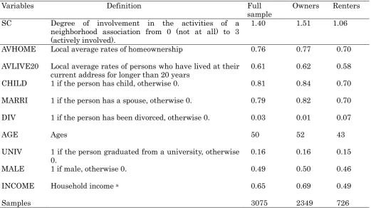
Variables used for the regression estimations are shown in Table 1; these include
variable definitions and mean values of all samples, as well as those of split samples
such as homeowners and renters. Homeownership is measured using the question
“What is your type of residence?” The responses were “I own my home”, “I reside in a
home owned by a parent” and “others”. I defined homeownership as being in a home
owned by individuals or their parents. The local group average value, AVHOME, is
incorporated as one of the independent variables. Furthermore, with a view to capture
the effect of the length of residence, I include AVLIVE 20 representing the local average
rates of persons who have lived at their current address for longer than 20 years.
AVHOME and AVLIVE20 are thought to capture the degree of population immobility in
a particular locality.
The view of Kan (2007) is that people integrated into neighbor ties are thought to be
inclined to invest in social capital since the return on investment is expected to be
sufficiently large. This seems to hold under conditions in which the individual’s barrier
to moving is high and ties with neighbors are strong. Individual barriers to moving are
captured by individual homeownership (DiPasquale and Glaeser 1999), while ties with
neighbors can be achieved from AVHOME and AVLIVE20. Therefore, AVHOME and
AVLIVE20 are predicted to take positive signs and their coefficients should become
larger when individuals are homeowners. Therefore, when estimations are conducted I
split samples into homeowners and renters. However, individuals who tend to invest in
social capital appeared to become homeowners, resulting in selection bias. Therefore, to
control for this bias, I also conducted Heckman’s sample selection estimation. In the
4
estimation, area dummies and metropolitan cities dummy as independent variables4. It
seems appropriate to argue that that area dummies and city size capture the local
housing market condition, leading me to assume that they are exogenous for an
individual’s decision on homeownership.
Following the model used by DiPasquale and Glaeser (1999), other independent
variables, such as marital status, demographic character, education, and household’s
income are included in the estimation function.
3. Estimation Results
Table2 sets out the estimation results. Column (1) shows the results using all samples.
For the purpose of comparing the effect on homeowners with that on renters, Columns
(2) and (3) present results of homeowner and renter samples, respectively. Column (4)
provides the results of Heckman’s estimation. I now restricted the results of AVHOME
and AVLIVE 20 to examine the argument as above.
In all estimations of AVHOME and AVLIVE20, as anticipated, all coefficient signs are
positive. As for all estimation results of the samples in column (1), both of AVHOME and
AVLIVE20 are statistically significant. Furthermore, the values of AVHOME and
AVLIVE20 are 0.97 and 0.47, respectively. It is interesting to observe that the value of
AVHOME in column (2), 0.90, is approximately 3 times larger than that in column (3),
0.34. Also, the value of AVLIVE20 in column (2), 0.50, is about 10 times larger than that
in column (3), 0.05. Furthermore, AVHOME and AVLIVE20 are statistically significant
in column (2), whereas they are insignificant in column (3). It follows from this that
neighbor immobility has a greater effect on homeowners than on renters. Heckman’s
5
estimation results are shown in column (4); revealing that after controlling for selection
bias, AVHOME and AVLIVE20 continue to take significant positive signs and the values
of AVHOME and AVLIVE20 are 0.85 and 0.48, respectively. This suggests that the
results of AVHOME and AVLIVE20 do not change, indicating that the estimation
results are robust5. What comes out of the findings above strongly supports the view
that the relationship between a neighbor’s barriers and an individual’s ones can be
considered complementary.
4.
Conclusion
The major findings of this analysis, which was based on the individual data, are as
follows; Neighbor immobility significantly enhances individual investment of
homeowners in social capital, whereas this neighbor effect on renters is not only smaller
but also statistically insignificant when samples are restricted to renters. From this, I
derived the argument that the neighbor immobility effect is increased by an individual’s
homeownership, and hence interaction between circumstances and an individual’s
characteristics has a critical role in social capital formation. Thus, I stress the
importance of simultaneously considering circumstances and individual characteristics
when analyzing incentives to invest in social capital.
There are no reports that have examined the relationship between neighbor
immobility and individual investment in social capital in other countries. As the
findings of this paper are naturally limited to the situation in Japan; it will, therefore,
be worthwhile exploring the extent to which these findings are valid under the different
5 In the first stage estimation, a dummy variable for metropolitan cities yielded a
7
References
Alesina, A, La Ferrara, E. 2000. Participation in heterogeneous communities. Quarterly
Journal of Economics 115(3), 847-904.
DiPasquale, D., Glaeser,E.L. 1999. Incentives and social capital: Are homeowners better
citizens? Journal of Urban Economics 45(2), 354-384.
Glaeser, EL, Laibson,D., Sacerdote, B. 2002, An economic approach to social capital.
Economic Journal 112, 437-458.
Hilber, C.A.L, 2007, New housing supply and the dilution of social capital. MPRA Paper
5134, (University Library of Munich, Germany).
Kan, K, 2007, Residential mobility and social capital. Journal of Urban Economics 61(3),
436-457.
Putnam, RD., 2000, Bowling alone: The collapse and revival of American community. (A
8
Table 1
Variable definitions and descriptive statistics
Note: a in 10 Million yen increments
Variables Definition Full
sample
Owners Renters
SC Degree of involvement in the activities of a neighborhood association from 0 (not at all) to 3 (actively involved).
1.40 1.51 1.06
AVHOME Local average rates of homeownership 0.76 0.77 0.70
AVLIVE20 Local average rates of persons who have lived at their current address for longer than 20 years
0.61 0.62 0.58
CHILD 1 if the person has child, otherwise 0. 0.81 0.84 0.70
MARRI 1 if the person has a spouse, otherwise 0. 0.79 0.82 0.70
DIV 1 if the person has been divorced, otherwise 0. 0.03 0.01 0.07
AGE Ages 50 52 43
UNIV 1 if the person graduated from a university, otherwise 0.
0.16 0.16 0.15
MALE 1 if male, otherwise 0. 0.49 0.50 0.46
INCOME Household income a 0.65 0.69 0.49
9 Table 2
Determinants of investment for social capital. Variables (1)
OLS All samples (2) OLS Homeowner (3) OLS Renter (4) HECKMAN
AVHOME 0.97** (5.08) 0.90** (3.93) 0.34 (0.92) 0.85** (2.68) AVLIVE20 0.47*
(2.15) 0.49* (1.92) 0.05 (0.13) 0.48* (1.84) CHILD 0.32**
(5.83) 0.29** (4.34) 0.32** (3.54) 0.29** (4.17) MARRI 0.16**
(3.14) 0.16** (2.62) 0.20* (2.05) 0.17** (2.63)
DIV -0.15
(-1.51) -0.16 (-1.16) -0.009 (-0.07) -0.14 (-0.87) AGE 0.01**
(9.32) 0.01** (7.42) 0.006** (2.73) 0.01** (4.36) UNIV -0.09*
(-2.06) -0.10* (-1.95) -0.09 (-0.96) -0.10* (-1.96) MALE -0.004
(-0.14) -0.003 (-0.09) -0.008 (-0.13) -0.003 (-0.09) INCOME 0.02
(0.73) -0.009 (-0.02) 0.13 (-1.25) -0.001 (-0.19)
Adj R- square 0.12 0.10 0.07
Wald chi- square 574
Sample size 3075 2349 726 3075
Uncensored sample 2349
10
1
1
.5
2
.4 .6 .8 1
homeowner