A Comparative Study of Locality Preserving Projection and Principle Component Analysis on Classification Performance Using Logistic Regression

http://dx.doi.org/10.4236/jdaip.2016.42005

A Comparative Study of Locality Preserving

Projection and Principle Component

Analysis on Classification Performance

Using Logistic Regression

Azza Kamal Ahmed Abdelmajed

Department of Computer Sciences, Faculty of Mathematical and Computer Sciences, University of Gezira, Wad Madani, Sudan

Received 6 March 2016; accepted 9 May 2016; published 12 May 2016

Copyright © 2016 by author and Scientific Research Publishing Inc.

This work is licensed under the Creative Commons Attribution International License (CC BY).

http://creativecommons.org/licenses/by/4.0/

Abstract

There are a variety of classification techniques such as neural network, decision tree, support vector machine and logistic regression. The problem of dimensionality is pertinent to many learning algorithms, and it denotes the drastic raise of computational complexity, however, we need to use dimensionality reduction methods. These methods include principal component anal-ysis (PCA) and locality preserving projection (LPP). In many real-world classification problems, the local structure is more important than the global structure and dimensionality reduction techniques ignore the local structure and preserve the global structure. The objectives is to com-pare PCA and LPP in terms of accuracy, to develop appropriate representations of complex data by reducing the dimensions of the data and to explain the importance of using LPP with logistic re-gression. The results of this paper find that the proposed LPP approach provides a better repre-sentation and high accuracy than the PCA approach.

Keywords

Logistic Regression (LR), Principal Component Analysis (PCA), Locality Preserving Projection (LPP)

1. Introduction

problems in the field of data mining [1]. Classification predicts categorical class labels and it classifies the data based on the training set and the values in classifying the attributes and uses it in classifying the new data. Data classification is a two-step process consisting of model construction and model usage. Model construction is used for describing predetermined classes. Model usage is used for classifying future or unknown objects [2]. The development of data mining applications such as classification has shown the need for machine learning al-gorithms to be applied specially in large scale data [3]. Machine learning focuses on the development of com-puter programs that can teach themselves to grow and change when exposed to new data; there are two types of machine learning: supervised learning and unsupervised learning: the first one is use training data to infer model and apply model to test data and for the other one, there is no training data, and model inference and application both rely on test data exclusively. Modern machine learning techniques are progressively being used by biolo-gists to obtain proper results from the databases. There are a variety of classification techniques such as neural network, decision tree, support vector machine and logistic regression. Logistic regression (LR) is a well-known statistical classification method that has been used widely in a variety of applications including document classi-fication, bioinformatics and analyzing a data set in which there are one or more independent variables that de-termine an outcome [4]. The advantage of using LR is that deals with dependent variables that are categorical and extension to the multiclass case. Logistic regression not just classes the data but also predicts probabilities and then estimates the parameters of the model using maximum likelihood estimator. Before using the data set in the classification, it needs some preprocesses such as data cleaning, data transformation and data reduction, the last one is very important because it usually represents the dataset in an (n*m) dimensional space, and these (n*m) dimensional spaces are too large, which however need to reduce the size of the dataset before applying a learning algorithm. A common way to attempt to resolve this problem is to use dimensionality reduction tech-niques [5]. Because principle component analysis (PCA) preserves the global structure of the dataset and ignores the local structure of the dataset. Therefore this paper proposes linear dimensionality reduction algorithm, called locality preserving projections (LPP). LPP is linear projective maps that arise by solving variational problem that optimally preserves the neighborhood structure of the dataset. LPP should be seen as an alternative to prin-cipal component analysis (PCA) [6]. This study aims to compare PCA and LPP in terms of accuracy, to develop appropriate representations of complex data by reducing the dimensions of the data and to explain the impor-tance of using LPP with logistic regression. A variety of performance metrics has been utilized: accuracy, sensi-tivity, specificity, precision, the area under receiver operating characteristic curve (AUC) and the receiver oper-ating characteristic (ROC) analysis. A detailed concept of using statistical analysis in comparing these methods is given.

2. Materials and Methods

2.1. Experimental Setup

In order to evaluate a prediction method it is necessary to have different data sets for training and testing, how-ever five datasets will be used and apply the algorithms principle component analysis (PCA) and locality pre-serving projections (LPP) to reduce the dimensions using dimensionality reduction toolbox (drtoolbox) in mat-lab software. After the input space is reduced to a lower dimension by applying one of the two methods PCA and LPP, cross-validation method will be applied to this new reduced features space using 10 fold to evaluation the model and then apply logistic regression to classifier the reduced data. All the performance measures: accu-racy, sensitivity, specificity, f-score, precision and roc curve will be computed. The ROC analysis is plotted after each cross validation for the two methods using spss software to compute the area under the curve.

2.1.1. Dimensionality Reduction Toolbox (Drtoolbox)

The template is used to format your paper and style the text. All margins, column widths, line spaces, and text fonts are prescribed; please do not alter them. You may note peculiarities. For example, the head margin in this template measures proportionately more than is customary. This measurement and others are deliberate, using specifications that anticipate your paper as one part of the entire journals, and not as an independent document. Please do not revise any of the current designations.

2.1.2. Cross Validation

evalua-tions is that they do not give an indication of how well the learner will do when it is asked to make new predic-tions for data it has not already seen. One way to overcome this problem is to not use the entire data set when training a learner. Some of the data is removed before training begins. Then when training is done, the data that was removed can be used to test the performance of the learned model on “new” data. This is the basic idea for a whole class of model evaluation methods called cross validation [7].

2.1.3. Performance Measure

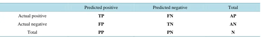
The measures that are used in this paper depend on matrix called the confusion matrix are as follows inTable 1: Where:

TP: true positives (predicted positive, actual positive), TN: true negatives (predicted negative, actual negative), FP: false positives (predicted positive, actual negative), FN: false negatives (predicted negative, actual positive) [8].

•Accuracy:

Accuracy is the proportion of true results (both true positives and true negatives) in the population [9].

TP+TN Accuracy=

TP+TN+FP+FN. (2.1)

•Sensitivity or Recall:

Proportion of actual positives which are predicted positive [9]

TP Sensitivity

TP FN

=

+ . (2.2) •Specificity:

Proportion of actual negative which are predicted negative [9]

TN Specificity

TN FP

=

+ . (2.3) •Positive predictive value (PPV):

Proportion of predicted positives which are actual positive [9]

TP Precision

TP FP

=

+ . (2.4) •F Score:

Harmonic Mean of Precision and recall [10]

(

)

2 Precision recall F Score=

Precision recall ⋅

+ . (2.5) •ROC analysis:

Receiver Operating Characteristics (ROC) graphs are a useful and clear possibility for organizing classifiers and visualizing their quality (performance) [10]. A Roc curve is a plot of TPR vs FPR for different thresholds θ. Receiver operating characteristic analysis is being used with greater frequency as an evaluation powerful me-thodology in machine learning and pattern recognition. The ROC is a well-known performance metric for eva-luating and comparing algorithms.

•Area under curve (AUC):

Table 1. Confusion matrix.

Predicted positive Predicted negative Total

Actual positive TP FN AP

Actual negative FP TN AN

AUC The area under the ROC is between 0 and 1 and increasingly being recognized as a better measure for evaluating algorithm performance than accuracy. A bigger AUC value implies a better ranking performance for a classifier [10].

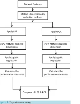
Figure 1 explains the Experimental Setup of this paper which uses any algorithm alone and then compares them.

3. Results and Discussion

3.1. Performance by Measures

Table 2 shows the classification results of the LR on the whole features, whileTable 3shows the classification results of logistic regression with principle component analysis algorithm.Table 4 shows the classification re-sults of logistic regression with locality preserving projection algorithm.

3.2. The ROC Analysis

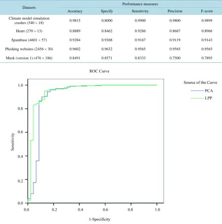
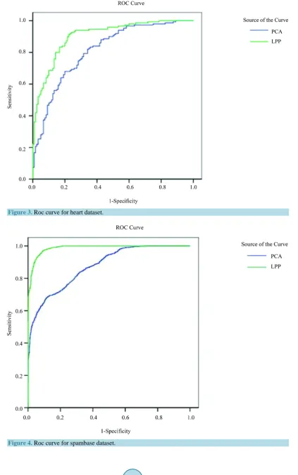
The estimated probability is used to construct the ROC analysis after each cross validation for the two feature selection methods.Figure 2 represents the PCA and LPP Roc curve for climate model simulation crashes data-set whileFigure 3 shows the PCA and LPP Roc curve for heart dataset.Figure 4 shows the PCA and LPP Roc curve for Spam Base dataset.Figure 5 shows the PCA and LPP Roc curve for Phishing Websites dataset. Fig-ure 6 shows the PCA and LPP Roc curve for Musk (version 1) dataset. The figures inTable 5 show the features selection methods; including PCA and LPP with LR; it shows that most points of AUCs of these methods for each dataset. However, the AUCs of LPP is higher for all data sets than PCA.

3.3. Discussion

Two experiments on five databases have been systematically performed. These experiments reveal a number of interesting points:

1) In all datasets Locality preserving projection approach performed better than principle component analysis. 2) The datasets is downloaded from UCI repository website and I selected this datasets because most of paper apply LPP on face recognition dataset and there in no study using normal datasets with LR and LPP, however it was necessary to compare LPP with another algorithm like PCA to show the different between them and to im-prove that LPP is the best than PCA.

3)Table 2 shows the results of the performance measures for logistic regression with all variables, while Ta-ble 3 shows the results of the performance measures for logistic regression with principle component analysis.

Table 4 shows the results of the performance measures for logistic regression with locality preserving projection. From those tables notice the locality preserving projection (LPP) method it has given a better result in all data sets although there are different in the number of Instances, number of attributes and type of attributes if com-pare to the principle component analysis (PCA) method and In all performance measures (accuracy, sensitivity, Specificity, precision, f-score and roc curve) LPP performs better than PCA.

4) The ROC curves of PCA, LPP with all data set are shown inFigures 2-5 and LPP seems to be the best one.

Table 5represents the AUCs of each data set and the value of the area under the curve in LPP bigger than the value in the PCA and that indicates to LPP is better than PCA.

5) Comparing to PCA method which it preserve the global structure, the LPP method preserving local struc-ture which is more important than the global strucstruc-ture for many reason: it is important to maintain the intrinsic information of high-dimensional data when they are transformed to a low dimensional space for analysis, a sin-gle characterization, either global or local, may be insufficient to represent the underlying structures of real world data and the local geometric structure of data can be seen as a data dependent regularization of the trans-formation matrix, which helps to avoid over fitting, especially when training samples are scarce.

4. Conclusion

Figure 1. Experimental setup.

Table 2. The results of the performance measures for logistic regression with all variables.

Datasets

Performance measures

Accuracy Specify Sensitivity Precision F-score

Climate model simulation crashes (540 × 18) 0.9259 0.7500 0.9400 0.9792 0.9592

Heart (270 × 13) 0.7778 0.7273 0.8125 0.8125 0.8125

Spambase (4601 × 57) 0.9067 0.9333 0.8571 0.8734 0.8652

Phishing websites (2456 × 30) 0.9283 0.9219 0.9350 0.9200 0.9274

Musk (version 1) (476 × 186) 0.7358 0.7500 0.7143 0.6522 0.6818

Table 3. The results of the performance measures for logistic regression with principle component analysis.

Datasets

Performance measures

Accuracy Specify Sensitivity Precision F-score

Climate model simulation

crashes (540 × 18) 0.9444 0.5000 0.9800 0.9608 0.9703

Heart (270 × 13) 0.8148 0.8333 0.8200 0.8571 0.8276

Spambase (4601 × 57) 0.9197 0.9296 0.9040 0.8889 0.8964

Phishing websites (2456 × 30) 0.9323 0.9329 0.9314 0.9048 0.9179

Musk (version 1) (476 × 186) 0.8113 0.8438 0.7619 0.7619 0.7619

Dataset Features

Apply LPP Apply PCA

Matlab (dimensionality reduction toolbox)

New featuresreduced dimensions

ApplyLogistic regression

Calculate the performance measures

New featuresreduced dimension

ApplyLogistic regression

Calculate the performance measures

Table 4. The results of the performance measures for logistic regression with locality preserving projection algorithm.

Datasets Performance measures

Accuracy Specify Sensitivity Precision F-score

Climate model simulation

crashes (540 × 18) 0.9815 0.8000 0.9900 0.9800 0.9899

Heart (270 × 13) 0.8889 0.8462 0.9286 0.8667 0.8966

Spambase (4601 × 57) 0.9284 0.9368 0.9167 0.9119 0.9143

Phishing websites (2456 × 30) 0.9602 0.9632 0.9565 0.9565 0.9565

Musk (version 1) (476 × 186) 0.8491 0.8571 0.8333 0.7500 0.7895

Figure 2. Roc curve for climate model simulation crashes dataset.

Figure 3. Roc curve for heart dataset.

Figure 5. Roc curve for phishing websites dataset.

Table 5. Area under the curve.

Datasets Methods

PCA LPP

Climate model simulation crashes 0.912 0.948

Heart 0.812 0.904

Spambase 0.847 0.966

Phishing websites 0.873 0.987

Musk (version 1) 0.792 0.899

5. Recommendations

This paper can be extended to other data mining techniques like clustering, association, it can also be extended for other classification algorithm such as neural network, decision tree and support vector machine and much more datasets should be taken. Moreover, this paper recommends by using more than mathematical model to obtain the best results.

References

[1] Rohit Arora, S. (2012) Comparative Analysis of Classification Algorithms on Different Datasets Using WEKA. Inter-national Journal of Computer Applications, 54, No. 13.

[2] Deepajothi, S. and Selvarajan, S. (2012) A Comparative Study of Classification Techniques on Adult Data Set. Inter-national Journal of Engineering Research & Technology (IJERT), 1, No. 8.

[3] bin Othman, M.F. and Yau, T.M.S. (2007) Comparison of Different Classification Techniques Using WEKA for Breast Cancer.

[4] Musa, A.B. (2013) A Comparison of ℓ1-Regularizion, PCA, KPCA and ICA for Dimensionality Reduction in Logistic Regression. International Journal of Machine Learning and Cybernetics.

[5] He, X.F., Yan, S.C., Hu, Y.X., Niyogi, P. and Zhang, H.-J. (2005) Face Recognition Using Laplacianfaces. IEEE Transactions on Pattern Analysis and Machine Intelligence, 27, No. 3.

[6] He, X.F. and Niyogi, P. (2004) Locality Preserving Projections (LPP).

[7] Murphy, K.P. (2007) Performance Evaluation of Binary Classifiers.

[8] Chaurasia, S., Chakrabarti, P. and Chourasia, N. (2014) Prediction of Breast Cancer Biopsy Outcomes—An Approach Using Machine Leaning Perspectives. International Journal of Computer Applications, 100, No. 9.

[9] François, D. (2009) Binary Classification Performances Measure Cheat Sheet.