Analysis, Design, and in vitro Implementation of Robust Biochemical Networks

(1)

Analysis, design, and

in vitro

implementation of robust

biochemical networks

Thesis by

Elisa Franco

In Partial Fulfillment of the Requirements

for the Degree of

Doctor of Philosophy

California Institute of Technology

Pasadena, California

2012

(2)

c

2012

Elisa Franco

(3)

(4)

Acknowledgements

My years at Caltech have been a true learning journey: I am grateful to many, many people for

accompanying me through it.

First of all, I want to thank my advisor Richard Murray, who made the journey possible and

provided me with invaluable guidance. His enthusiasm, support, and vision turned into exciting

chal-lenges many of what I thought were research dead ends or unsurmountable issues. I am very grateful

to Erik Winfree, who generously allowed me to become an extended member of his laboratory. His

sharp ideas, constructive criticism, and amazing attention to detail have been essential stepping

stones for the development of my graduate work. I would also like to thank Paul Rothemund and

John Doyle for being part of my thesis committee.

My deepest gratitude goes to Jongmin Kim, for introducing me toin vitro synthetic circuits and

being a wonderful collaborator and friend for many years. I am also thankful to all the members of

the Winfree lab, and in particular to Nadine Dabby, Rebecca Schulman, and Rizal Hariadi for their

support, feedback, and friendship.

I am in great debt to my friend Franco Blanchini: he helped turn a casual conference hallway

conversation into a good research project. I also want to thank Domitilla Del Vecchio for helpful

discussions and advice. I am grateful for having collaborated with John Dabiri at the beginning of

my graduate studies.

I was lucky to work with bright and curious undergraduates: Per-Ola Forsberg, with whom I

started the flux regulation project, Chris Sturk, and Fei Chen.

All the members of the Murray group have been extraordinary journey companions – literally so,

during the fun and adventurous Murray group trips. In particular, I want to thank Mary Dunlop,

Julia Braman, Vanessa J¨onsson, Ophelia Venturelli, Tim Chung, Pete Trautman, Marcos Nahmad,

Dionysios Barmpoutis, and Shuo Han. I am also in debt to Dennice Gayme and Genti Buzi for

our “job search” sessions, and to Katie Galloway and Josh Michener for the stimulating bio-control

journal club meetings.

For helping with laboratory supplies, traveling, and many other the practical details of my

doctorate years, I am grateful to Gloria Bain, Karolyn Knoll, and Anissa Scott.

(5)

harder process: in particular, I would like to thank Daniela Maniezzo, Maria Rita D’Orsogna,

Guido Maretto, Roberto Congiu, Martina Carbone, Diego Fazi, Pierpaolo Bergamo, Luca Giacchino,

Riccardo Schmid, Andrea Censi, and Luigi Perotti.

Finally, I have to thank my family for their endless support. In particular, my mother Marina,

my aunt Lucia, and my husband Mohsen, for their love and patience; and my old friend Tariq for

(6)

Abstract

The functionalities of every living organism are wired in the biochemical interactions among

pro-teins, nucleic acids, and all the other molecules that constitute life’s building blocks. Understanding

the general design principles of this “hardware of life” is an exciting and challenging task for modern

bioengineers. In this thesis, I focus on the topic of molecular network robustness: I investigate

several design rules guaranteeing desired functionalities in specific systems, despite their

compo-nents variability. Experimental verifications of such design schemes are carried out using in vitro

transcriptional circuits, a minimal analogue of cellular genetic networks.

The first problem I consider is flux control, which is a fundamental feature for the correct

performance of biochemical systems. I describe a simple model problem where two reagents bind

stoichiometrically to form an output product. In the absence of any regulation, imbalances in the

reagent production rates can cause accumulation of unused molecules, and limit the output flow. To

match the reagents’ flux robustly with respect to the open loop rates, I propose the use of negative

or positive feedback schemes that rely on competitive binding. Such schemes are modeled through

ordinary differential equations and implemented using transcriptional circuits; data are presented

showing the performance of the two approaches.

The second topic I examine is the functional robustness of interconnected networks. Molecular

devices characterized in isolation may lose their properties once interconnected. This challenge

is illustrated with a case study: a synthetic transcriptional clock is used to time conformational

changes in a molecular nanomachine called DNA tweezers. Mass conservation introduces parasitic

interactions that perturb the oscillator trajectories proportionally to the total amount of tweezers

“load”. To overcome this problem, we can use a transcriptional switch that acts as a buffer amplifier,

achieving signal propagation and at the same time reducing the perturbations on the source of signal.

Finally, I describe a general class of control-theoretic methods to analyze structural robustness

in natural biological systems. Using Lyapunov theory and set invariance, the stability properties

of several well-known case studies are analytically demonstrated. The key feature of this analysis

is its reliance on parameter-independent models, which only capture essential dynamic interactions

(7)

Introduction

1.1 Design principles for robust molecular networks

All living organisms, from bacteria to humans, share a remarkable feature: to survive, they must

be able to sense external stimuli and implement adequate responses. The ability to effectively

control their own behavior based on the “measured” environment is what makes individuals fit and

successful. But how do living things make decisions that are crucial to their survival? This question

branches out in many directions: from neuro-economics to ethology to molecular biology, several

research fields have focused on different aspects of how “control” happens at every layer of what we

call life.

At the simplest level, we find that single cells are individually capable of interacting with their

surroundings: in this context, decision making and control are embedded in biochemical events. One

of the most classical examples is given by the famous experiments of Jacob and Monod [53] in the

1960s, which showed thatE. coli adapts its gene expression profile to the type of nutrient available.

When lactose is abundant, but glucose is not, a set of genes called the lac operon is activated

through a lactose-dependent cascade of reactions. The proteins expressed from thelacoperon allow

the cells to metabolize lactose and grow. In the absence of lactose, or when glucose is present at

high concentrations, thelac operon genes are repressed: thus, cells do not waste energy to produce

unnecessary lactose-digesting enzymes. This is a clear example of how the control center of a cell is

in large part constituted by chemical reactions. It is appropriate to classify a set of molecules that

interact and thereby induce specific cellular behaviors as a molecular or biochemical network.

Continuing with our example, the metabolites, genes, and proteins involved in the lac operon

genetic switch should respond consistently to variations in the available nutrient. However, cells

generally differ from each other in size, and therefore in the number and distribution of metabolites

and proteins present. Moreover, the intracellular environment is crowded and its content is affected

by several parameters, such as temperature and external inputs. Potentially, undesired interactions

(11)

network behavior.

So are there features that confer robustness to a biochemical network? Although evolution

op-erates more as a tinkerer than as an engineer [6], several examples of engineering design principles

have been identified in biological systems. For example, negative feedback is the control theorists’

favorite tool to confer robustness to a system [12], because it structurally reduces the impact of

parametric uncertainty and disturbances. In the biological world, there is evidence that negative

auto-regulation in gene expression reduces the variability of protein concentration in cellular

popu-lations [16]. Negative feedback has also been related to the response robustness (and speed) of the

heat shock response inE. coli [31].

A classical example of robust molecular circuitry is probably given by bacterial chemotaxis [14,

9, 117]. The action of the flagellar motor ofE. coli is driven by a cascade of signaling proteins, whose

active or inactive state is determined by the presence of nutrient in the environment. Both analysis

on a simplified ordinary differential equation (ODE) model [14] and experiments [9] showed how the

E. coli flagellar motion presents a robustly stable steady-state: steps in the nutrient concentration

only temporarily alter the motor equilibrium. Cells are therefore sensitive to nutrient gradients,

but always return to their steady state motion (such property is also referred to as adaptability).

Such stable steady state can be described as a function of the concentrations of the signaling

cas-cade protein components and a few binding rates, and is therefore independent of external inputs.

Further analysis also demonstrated how integral feedback is present in the chemotaxis network, and

guarantees robustness (perfect adaptation) of the equilibrium [134].

Experimental and theoretical studies aimed at unraveling the design principles of existing

biologi-cal networks generally fall under the category of systems biology. A different approach is represented

by synthetic biology [87], which instead focuses on the design of new biological circuits. However,

creating new functionalities can be also useful for probing existing systems. On the one hand, for

instance, bacteria and yeast have been engineered to become micro-scale factories to produce fuel,

anti-malarial drug precursors, insulin, and even silk [69, 100, 131]. On the other hand, we can cite

the example of the MAPK pathway synthetic re-wiring, which has been extremely helpful in

clari-fying the role of several proteins involved in the cascade [17, 15]. Another class of examples is given

by the many artificial oscillators synthesized in the past decade [13, 25, 33, 44, 128], which provide

insights into the design principles underlying natural cellular clocks and circadian rhythms.

Robust-ness of negative-feedback-loop-based oscillators, for instance, has been experimentally linked to the

presence of delays [122], in agreement with classical control theory results [99, 11]. The synthetic

approach has also given interesting insights regarding organism-level network robustness: in [52],

for instance, it was demonstrated that survival ofE. coli was not significantly altered by promoter

recombinations adding new links across different networks. Some of the re-wired networks actually

(12)

It is imperative to characterize and study molecular networks in their own operational context,

the cell. However, the complexity of the cellular environment may be an insurmountable obstacle to

a detailed understanding of molecular interactions. In fact, quantitative predictions on the dynamic

behaviors of in vivo molecular networks are limited to small systems, mostly due to the lack of

knowledge of the system parameters and to the presence of unmodeled reactions. Synthetic, cell-free

biochemical approaches offer a bottom-up, simplified alternative to the study of molecular circuitry.

1.2 Cell-free methods

Operating in an in vitro environment with a limited number of biological parts offers several

ad-vantages. First, many layers of complexity present in vivo may be eliminated, allowing scientists

to focus on specific phenomena more quantitatively. Second, fully artificial biological design

princi-ples and chemistries can be explored, opening new doors for technology and for understanding the

evolution of life.

Cell-free transcription and translation regulatory circuits have been successfully reproduced

in [90], with the purpose of achieving a high level of detail (relative to in vivo studies) in the

investigation of genetic network behaviors. A good example of howin vitro assays can reveal new

information about natural networks is given by [88], where the reconstruction of circadian

oscilla-tions of cyanobacterial KaiC phosphorylation showed that this process is independent of

transcrip-tion and translatranscrip-tion. Recently, a similar in vitro set of experiments showed that the dynamics of

this oscillator are determined by intermolecular associations: for instance, mutations altering the

binding rates of KaiB to KaiC will modulate the oscillator period [96]. A faithful reproduction

of in vitro cellular environment is still challenging, requiring many components [112] or

not-well-characterized extracts [90]. However, transcription-translation kits for cell-free protein production

are now commercially available; such kits are particularly useful for the synthesis of unnaturally

modified aminoacids [114, 113].

The quest for the minimal biochemistry that supports life [125, 73] is another area wherein vitro

experiments are essential. A related topic of great interest is the role of nucleic acids in general, and

of RNA in particular, in the development of life and regulation of gene expression [38, 22].

In vitro synthetic biology and nanotechnology are rapidly evolving [119, 30] in many directions:

one relevant trend is the use of nucleic acids for the implementation of natural algorithms and

chemical reaction networks. The most attractive property of nucleic acids is programmability [118]:

established methodologies are available to reliably predict structure and hybridization pathways of

an oligonucleotide molecule, starting from its plain sequence information [141, 80, 2, 28]. If we

can predict the structure of a given nucleic acid strand, the ability to design systems of strands

(13)

nucleic acids have been designed to self-assemble into arbitrary shapes [102, 59]; to create devices

moving on programmed paths [74, 137] and performing tasks [47]; and to construct biochemical logic

circuitry [110, 140] and molecular machines [139, 24].

The programmability of nucleic acids makes them an ideal candidate for theoretical and

experi-mental studies regarding general chemical reaction networks. In [120], the authors propose motifs for

the implementation of arbitrary chemical dynamics with nucleic acids: such dynamics are generated

through toehold-mediated branch migration [138, 111], and their speed can be tuned by suitably

choosing the length of the toehold domains. (I will return to the topic of branch migration in

Sec-tion 1.2.1.) Numerical tools for the automated generaSec-tion of DNA strands implementing a desired

reaction network are also available [93].

Although nucleic acid catalytic devices are available, it is interesting to explore the computational

and dynamical capabilities of systems integrating proteins and nucleic acids. This is an attractive

setup for two main reasons: first, we have a chance to work with molecular network scenarios that

may be closer to those of natural networks; second, we can develop useful ground knowledge for

the simultaneous programmability of both nucleic acids and amino-acid sequences. Predicting and

programming enzyme folding and function is a very active research area [77]: however, custom

protein synthesis (with a specified structure and function) is still not possible.

One of the first attempts to constructin vitromolecular circuitry using DNA and proteins is the

predator-prey system in [4], which consisted of DNA templates and only three proteins: T7 RNA

polymerase, M-MLV reverse transcriptase, and RNase H cloned from E. coli. The accumulation

of sequence mutations is one of the likely reasons for the limited success of those experiments.

More recently, logic gates using several enzymes [126] and full metabolic platforms [55] have been

characterized. Transcriptional circuits, developed by J. Kim in the Winfree lab at Caltech, are a

versatile tool for building molecular networks, and will be described in detail in the next section.

1.2.1 In vitro

transcriptional circuits

Synthetic in vitro genetic transcriptional circuits [61, 63] consist of nucleic acids and two protein

species, T7 RNA polymerase (RNAP) and E. coli RNase H. Here I will describe their general

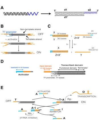
features, providing the relevant background information for Chapters 2 and 3 of this thesis. Starting

with Figure 1.1 A, from now on nucleic acids will be graphically represented as linear strings of

letters corresponding to their bases (the helical geometry of double-stranded DNA and RNA will

not be shown); the backbone 5’-3’ direction will be indicated with an arrow at the 3’ end. When

appropriate, specific functional areas, or domains, of a nucleic acid strand will be associated with

different colors (e.g., domains d1 and d2 in Figure 1.1 A); complementary strands will have the same

color (e.g., domains d1 and d1’ in Figure 1.1 A).

(14)

A

B

C

D

TGAACGAACGACACTAATG

!

AACTAC

GTAGTTCATTAGTGTCGTTCGTTCA

!

GTGTAGTGTTG

d1 d2

d1’

E

ON OFF + activator

T7 promoter

+

k+

k-35 bases

C=A’

C=A’ A

B

35 bases

25 bases

A B

∆G -60kcal/mol

∆G -40kcal/mol X

Y Z=X’

Z=X’ X

Y

Terminator

toehold 4-10 bases Consensus domain _{17-20 bases}

T7 promoter, 17 bases

Transcribed domain

Functional domain

Activator

OFF _ON

ACTIVATOR

INHIBITOR

TRANSCRIPTION Rp

Rh (if RNA inhibitor)

-12

+1

A

I

T T•A

O

A A•I

A

Template strand Non-template strand

Input domain

5’ 3’

30 bases

[image:14.612.150.498.81.502.2]

-50kcal/mol

(15)

one (or more) inputs and generating one (or more) outputs, which can be used to interconnect

different switches [61]. Such switches can be implemented as short, linear, synthetic genes whose

activity can be turned on and off by altering their promoter region. From now on I will refer to

these short artificial genes in transcriptional networks as templates or “genelets”, a term originally

suggested by Prof. E. Klavins. I will now introduce two notions that are helpful for understanding

how the state of such genelets can be systematically switched.

•Switching promoter activity: Promoters are double-stranded genetic domains having a high

binding affinity for RNA polymerase. The binding affinity can be lost when the structure [57] or

sequence [49] of the promoter region is altered, resulting in weaker transcription of the downstream

region. A promoter that is partially single-stranded, where the template strand is missing, does

not represent a good binding site for RNAP [57]. Referring to Figure 1.1 B, top, if the non-coding

strand of the promoter is single-stranded, the genelet can be effectively considered off. The

tran-scription rate of this incomplete promoter is, in general, below 10% of the trantran-scription rate of

a fully double-stranded promoter. This residual transcription activity is here called transcription

“leak”, and we find that it is dependent on the promoter flanking sequences 3.7.13. When a DNA

strand complementary to the promoter single-stranded domain is added in solution, the

transcrip-tion efficiency is recovered and the gene can be considered on. (Data comparing the on and off

transcription efficiency of some of the genelets used in this thesis are shown in Section 3.35.) The

single-stranded DNA species switching on the genelet will be called an activator. Details regarding

the optimal design of the nicked promoter can be found in [61], Section 3.4. So far, only the

bacte-riophage T7 promoter has been used in transcriptional circuits, due to its high binding affinity and

transcription efficiency for the T7 RNA polymerase enzyme, which is commercially available from

most biotechnology vendors.

•Branch migration: Consider the two nucleic acid complexes shown in Figure 1.1 C, top. One is formed by strands X and Y, the second is a single-stranded species Z, which is fully complementary

to X. The complex formed by strands X and Y is partially single-stranded: the blue overhang

is an exposed domain, to which the corresponding blue domain of strand Z will initiate binding,

subsequently peeling off X from Y. In fact, the system switches quickly to a final, thermodynamically

more favorable configuration, where X is bound to its complement Z=X’ and Y is released in solution.

The blue overhang, where the migration of strands is initiated, is called a toehold. The speed of

the reaction is determined by the length of the toehold, as shown in [138] through fluorescence

experiments.

The two above notions can be combined: a genelet may be designed to be switched on by

an activator strand added in solution, and switched off by branch migration. Branch migration

(16)

complex, stripping off the activator strand. General genelet design specifications for the required

domains and their lengths, are shown in Figure 1.1 D. The overall mechanism for switching on and

off a genelet is depicted in Figure 1.1 E.

Genelets can be interconnected through their RNA outputs by means of an inhibition or

acti-vation pathway. The RNA output of a genelet can serve as an inhibitor for a downstream genelet;

alternatively, the RNA output can be used to release an activator otherwise sequestered in an

ac-tivator/inhibitor complex. RNA has the potential to activate a DNA template by binding to the

single-stranded activation domain, thereby completing the promoter; however, due to the constraints

of our system, this is pathway is not used [82]. Degradation is introduced in the system using the

endonuclease RNase H, which targets DNA-RNA hybrids, hydrolyzing the RNA strand and releasing

the DNA strand.

The general theoretical foundations for transcriptional circuits were laid out in [62], where the

computational capability of these molecular networks is demonstrated to be equivalent to that

of neural networks. In general, it is possible to systematically model these circuits using ODEs.

(Typically, transcriptional circuits experiments are run at high molecular counts: stochasticity can

be safely neglected.) For instance, referring to Figure 1.1 E, consider a genelet T having a DNA

activator A, an RNA inhibitor I, and an RNA output O. The chemical reactions expected to occur

by design are:

Activation T + AkTA

→ T_·A

Inhibition T_·A + IkTAI→ T + I_·A

Annihilation A + IkAI

→A·I

Transcription: on state RNAP + T_·A

k+_ON → ← k−_ON

RNAP_·T_·AkcatON

→ RNAP + T_·A + O (1.1)

Transcription: off state RNAP + T

k+_OFF → ← k−_OFF

RNAP_·TkcatOFF

→ RNAP + T + O

Degradation RNaseH + A_·I

k+_H → ← k−_H

RNaseH_·A_·IkcatH

→ RNaseH + A.

(All hybridization reactions are reversible, but the reverse reaction is extremely slow and can be

neglected in practice.) The corresponding ODEs can be derived immediately, following the general

rules for mass action kinetics. In general, nucleic acid hybridization rates can be measured or

estimated from the literature, while enzymatic parameters are more difficult to establish and have a

higher variability [61, 63, 64]. (Enzymatic parameter uncertainty will be discussed in particular in

(17)

The concentrations of activators and inhibitors represent tunable thresholds. Branch

migra-tion reacmigra-tions yielding inhibimigra-tion, annihilamigra-tion, or activamigra-tion are stoichiometric, competitive binding

processes. Competitive binding easily generates ultrasensitive responses of the switches [21, 81]:

this is an important design feature of transcriptional circuits, and is particularly crucial to achieve

oscillatory dynamics.

Several networks have been experimentally characterized using transcriptional circuits:

self-inhibiting and self-activating genelets [61], a bistable toggle switch [63], and negative-feedback-based

oscillators differing for their topology [64]. In this thesis, I will use this tool kit to construct systems

achieving robust properties to be defined later.

1.3 Thesis overview and contribution

Let us go back to our initial question: what are the features that confer robustness to a biochemical

network? In this thesis, I will focus on three different topics related to this question. Two chapters

include work that follows a “synthetic”, bottom-up approach: I will consider specific robust design

objectives for biochemical networks, followed by synthesis using transcriptional circuits. The last

chapter will instead follow a “systems” approach, reporting more general theoretical robustness

results for existing molecular pathways.

•Chapter 2: Flux control for molecular networks. Flux control is a fundamental feature

for the correct performance of large scale networks, of which familiar examples are the Internet,

power grids, or even pipe networks. In the biological world, cells rely as heavily for their survival

on a regulated flow of nucleic acids, transcription factors, and other metabolites. It is therefore

interesting to explore and understand molecular flow rate control at the molecular level, especially

to develop systematic design principles for large biochemical circuits.

In this chapter I will propose two network architectures based on negative and positive feedback, to

regulate and match the output flow rate of two interconnected systems. Feedback is implemented

through mass action chemical reactions, which down- or up-regulate the activity of the molecules

generating the network output. To my knowledge, this design has not been considered elsewhere

in the literature. First, negative auto-regulation and positive cross-regulation will be introduced

through a very simple, intuitive ODE model. Then, I will describe the implementation of these

networks using transcriptional circuits, showing preliminary experimental results. Numerical

sim-ulations and data suggest that feedback confers robustness to the system with respect to certain

parametric variations and to initial conditions.

The general idea of flux control through positive and negative feedback has been previously presented

(18)

the negative auto-regulation circuit; the first experiments and numerical simulations were carried

out by an undergraduate student, Per-Ola Forsberg (SURF program at Caltech). Richard Murray

suggested studying the cross-activation scheme. All the analysis, data, and numerical simulations

reported in this thesis were performed by me.

•Chapter 3: Modularity of interconnected systems. An important research direction in

synthetic biology is the systematic design and construction of large molecular networks. Ideally,

biological devices should behave modularly, i.e., they should maintain their functionalities

(charac-terized in isolation) when interconnected to other devices. This can be rephrased as a question of

robustness: by design, the properties of a system should not be disrupted by the interconnection with

other systems. Achieving modularity is a challenge in most engineering fields: classical examples

include voltage drops at the output of non-ideal voltage generators, pressure losses in pipe networks

and level changes in systems of tanks.

This chapter is dedicated to the experimental study of a molecular oscillator to be used as a clock for

a downstream molecular device. Mathematical modeling and experiments show that interconnecting

the oscillator to its load in a direct manner, i.e., by stoichiometric binding and release, results in

undesired back-action effects and loss of the original signal. Loosely speaking, the back-action is

primarily caused by mass conservation constraints. This issue is mitigated by the introduction of a

molecular insulator, a node draining a small amount of molecules from the oscillator and using them

to amplify its signal [27]. Experiments are carried out using the tool kit of transcriptional circuits.

The project presented in this chapter was developed in close collaboration with the group of Prof.

Friedrich Simmel at the Technical University in Munich. F. Simmel and E. Friedrichs had the original

idea of using the transcriptional oscillator proposed in [64] to time conformational switching in the

well-known molecular tweezers system [139]. Jongmin Kim initially suggested connecting another

genelet to the oscillator, using its RNA output to induce switching in the tweezers; this eventually

became our insulator design. My contribution was the idea of using this system as a benchmark to

study the general challenges of molecular modularity and insulation; such idea was largely inspired

by [27] and by several discussions with Prof. Domitilla Del Vecchio. While several experiments I

performed were originally designed by the group at TUM, I developed many control experiments to

better understand the retroactivity effects and the tweezers behavior. Specific challenges I tackled

were data reproducibility, oscillation frequency and amplitude tuning, and the development of a

new transcription protocol to avoid the use of commercial kits. In this thesis I will only report

experiments performed by me at Caltech, unless explicitly noted in the text or figures. I also

contributed the analysis on the simplified model system illustrating the challenge of retroactivity in

Section 3.2. Detailed first principles models and parameter fitting were performed by J. Kim and

(19)

context of transcriptional circuits was also presented in [39].

•Chapter 4: Robust properties of natural networks. As already noted, the molecular

circuitry of living organisms performs remarkably robust regulatory tasks, despite the intrinsic

vari-ability of its components. A large body of research has in fact highlighted that robustness is often

a structural property of biological systems. However, there are few systematic methods to

mathe-matically model and describe structural robustness. With a few exceptions, numerical studies have

been thede facto standard for this type of investigation.

In this chapter I will highlight how robust stability of equilibria in biological networks can be

analyzed using Lyapunov and invariant sets theory. In particular, the analysis is focused on the

structure of ODE models rather than on their specific functional expressions. Without resorting to

extensive numerical simulations, the stability properties of well-known biological networks will be

rigorously proved to be robust. Several case studies will be considered, including thelacoperon and

the mitogen-activated protein kinase (MAPK) pathway.

This project was developed with Prof. Franco Blanchini at the University of Udine. F. Blanchini

and I conceived together the general idea of structural analysis of biological models using Lyapunov

functions. F. Blanchini mainly focused on the technical results; I contributed the models and assessed

the key assumptions and interpretations of the results in a biological context. This chapter reports

(20)

Chapter 2

Flux control for biochemical

networks

2.1 Introduction

Cellular pathways rely heavily on a regulated flux of nucleic acids, transcription factors, and other

metabolites. In the era of synthetic biology, it is important to understand and optimize the

mecha-nisms that control and optimize molecular flows. This will contribute to the formulation of systematic

design rules for constructing large biochemical networks [92]. (In the following I will use the words

flux and flow interchangeably.)

Here, I will consider a simple model problem: given two reagents that bind to form a product,

how can we equate their flow through the design of suitable feedback loops? If the two flows are

not matched, we could fall in a scenario where (1) the reagent with the higher flux will accumulate,

creating a potentially harmful excess of such species and (2) the flow of product will be limited by

the lower reagent flux. Two different network design solutions to these problems will be proposed,

both based on the use of feedback. A desirable feature of such designs would be their robustness

(low sensitivity) with respect to the open loop production rate of the reagents.

The first scheme relies on the use of negative auto-regulation: either species in excess is designed

to down-regulate its own production rate. Situation (1) is therefore avoided. The second scheme is

based on positive cross-regulation: if one of the reagents is in excess, it will increase the production

rate of the second reagent. This second architecture aims at avoiding point (2). The main feature

of both these schemes is that feedback is implemented using stoichiometric reactions and without

making time-scale separation arguments, which typically yield Michaelis-Menten or Hill functions.

The flux-matching problem and the outlined solutions will first be described with a simple

sys-tem of ODEs. Then, I will outline how the properties of these feedback schemes can be assessed

experimentally using transcriptional circuits. Experiments on the implementation of the negative

(21)

flow-matching is achieved robustly with respect to the open loop rates. On the contrary, the positive

cross-regulatory scheme presents several design challenges and the data currently available do not

verify the flux matching property conclusively.

2.2 Problem formulation

Consider a simple chemical reaction network

T1

β1

*R₁+ T₁,

T2

β2

*R2+ T2,

R1+ R2 k

*P. (2.1)

Two chemical species T1 and T2 produce, respectively, reactants R1 and R2, at rates β1, β2. The

reactants then bind to form an output product P. T1 and T2 could be, for instance, two genes

whose mRNA or protein outputs R1 and R2 must interact stoichiometrically to form a complex

useful for a downstream process. A pictorial representation of the network is given in Figure 2.1 A.

The differential equation corresponding to the dynamics of Ri is:

d[Ri]

dt =βi·[Ti]−k [Ri][Rj], i,j∈ {1,2},i6= j. (2.2)

The build-up of the product P is clearly conditioned by the ratesβ1, β2 and the concentrations

[T1] and [T2]. If the production rates for R1 and R2 are significantly different, one can make two

observations. First, the reactant produced at the higher rate will accumulate in the system. Second,

the lower production rate becomes a bottleneck for the formation of P. For instance, if [T1][T2], the concentration of R2builds up; at the same time the yield of P is limited by the production rate

of R1. If reactions (2.1) represent a genetic circuit in a cellular host, an excess of R2could harm the

organism, besides causing a waste of resources. Ideally, biochemical or metabolic networks should

include feedback loops able to eliminate excess production of molecules that are not utilized by the

system, and increase insufficient production of molecules in high demand. The solution trajectories

for equation (2.2) are shown in Figure 2.2. Parameters were chosen asβi= 0.01/M, k = 2·103/M/s, T1= 100 nM, T2= 200 nM.

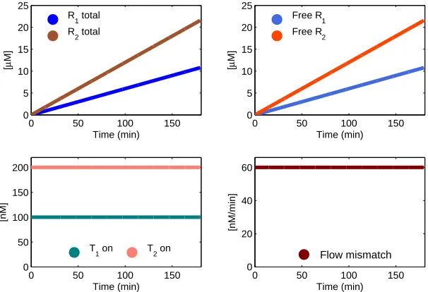
In this work, I will consider the model system (2.1) when the production rates for Ri are not

balanced. The question that will be asked is: If we could design R1 and R2 to interact with the

generating species T1 and T2, could we achieve self-regulation and matching of the flux rates for

the two reactants, robustly with respect to the open loop rates? I will investigate this question by

looking at the effects of the feedback loops that can be generated by R1and R2. In particular, I will

(22)

B

A

C

T₁ R1

R₂ T2

P

T1 R1_R

2 T2

P [R1]>[R₂]

[R2]>[R1]

T1 R1_R

2 T2

P [R1]>[R₂]

[image:22.612.174.477.248.455.2]

[R2]>[R₁]

Figure 2.1: A. Schematic representation for our model problem (2.1). B. Negative feedback scheme to control the flow of R1 and R2, corresponding to equations (2.3). The comparison between the concentrations of R1 and R2 is implicit, due to the formation of the product P. C. Positive feedback interconnection to control the flow of R1 and R2, corresponding to equations (2.7).

0 50 100 150

0 50 100 150 200

Time (min)

[nM]

T₁ on T₂ on

0 50 100 150

0 5 10 15 20 25

Time (min)

[

µ

M]

Free R₁

Free R 2

0 50 100 150

0 5 10 15 20 25

Time (min)

[

µ

M]

R₁ total

R

2 total

0 50 100 150

0 20 40 60

Time (min)

[nM/min]

Flow mismatch

Figure 2.2: Numerical solution to the differential equations (2.2). Bottom right: absolute value of the flux mismatch between the total amount of species Rtot1 and Rtot2 .

(Figure 2.1 C). I will assume that the feedback occurs by mass action chemical reactions.

2.2.1 Self-repression

Free molecules of Ri, i = 1,2, bind to active Ti thereby inactivating it:

Ri+ Ti

δi *T∗_i,

T∗i

αi *_T_i_,

where T∗_i is an inactive complex. We assume that Ttot

i = Ti+ T∗i, and that T∗i naturally reverts to

its active state with a first-order rate αi. The total amount of Ri is [Rtoti ] = [Ri] + [T∗i] + [P]. A

(23)

differential equations are:

d[Ti]

dt =αi([T tot

i ]−[Ti])−δi[Ri][Ti], d[Ri]

dt =βi[Ti]−k [Ri][Rj]−δi[Ri][Ti]. (2.3)

For illustrative purposes, the above differential equations are solved numerically. The parameters

chosen are: α1=α2= 3·10−4 /s,β1=β2= 0.01 /s,δ1=δ2= 5·102 /M/s, and k = 2·103/M/s. An imbalance in the production rates of R1 and R2 is created by setting [T1](0) = [Ttot1 ] = 100 nM

and [T2](0) = [Ttot2 ] = 200 nM, while [R1](0) = [R2](0) = 0. The overall result of this feedback

interconnection is that the mismatch in the flow rate of R1and R2is reduced, as shown in Figure 2.3.

The flow rate is defined as the derivative of the total amount of [Rtot

i ]. The flow rate mismatch is

defined as the absolute value of the difference between the two fluxes. The effect of changing the

feedback strength, for simplicity chosen as δ1 = δ2, is shown in Figure 2.4: the figure shows the

mean active fraction of [Ti] and the mean flow mismatch over a trajectory simulated for 10 hours.

The mean is shown, rather than steady-state values, to capture the behavior of the system over the

whole trajectory.

It is possible to examine the nullclines relating T1 and ¯T2, and find the equilibria ¯T1and ¯T2 as

intersection of these nullclines:

˙

Ti = 0 =⇒ Ri =

αi(Ttoti −Ti)

δiTi

,

˙

Ri= 0 =⇒ Ri =

βiTi kRj+δiTi

.

To simplify the derivation, we set δ1 = δ2 = δ, β1 = β2 = β, α1 = α2 = α. Equating the two

expressions forRi, we get the following equations (for i= 1,2 andj= 1,2):

α

δ 2

k _Ttot

i −Ti Ti

_Ttot

j −Tj Tj

!

+α(Ttoti −Ti)−βTi = 0.

We can find an expression of the nullclines by introducing a change of variables u =Ttot1 −T1

T1

and

v =Ttot2 −T2

T2

, and defining φ1 =ψ1 = α_δ 2

k, φ2 =αTtot1 , ψ2 =αTtot2 , φ3 =βTtot2 , and finally

ψ3=βTtot1 :

u2(φ1v) + u(φ1v +φ2−φ3 1

1 + v)−φ3 1

1 + v = 0, (2.4)

v2(ψ1u) + v(φ1u +ψ2−ψ3 1

1 + u)−ψ3 1

(24)

The roots of the equations above represent the nullclines of the system. Because all the

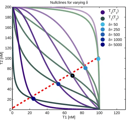
param-eters in these equations are positive, there is always a single root. The nullclines are numerically

solved, for varyingδ, in Figure 2.5.

A condition for flow matching at steady-state can be derived as follows:

˙

R1−R˙2= 0,

β1T1−δ1T1R1=β2T2−δ2T2R2.

Substituting the expressions for R1 and R2 that can be derived by setting ˙T1= 0 = ˙T2, we get:

β1T¯1−α1(Ttot1 −T¯1) =β2T¯2−α2(Ttot2 −T¯2).

Takingα1=α2=α, β1=β2=β we get:

¯

T2= ¯T1+

α

α+β(T

tot

2 −T

tot

1 ). (2.6)

The flow matching condition above is shown in Figure 2.5, red dashed line. If β α, i.e., the production of Ri is much faster than the generating species Ti inactivation rate, then the condition

can be rewritten as:

¯ T1≈T¯2.

0 50 100 150

0 50 100 150 200

Time (min)

[nM]

T

1 on T2 on

0 50 100 150

0 0.5 1 1.5

Time (min)

[

µ

M]

Free R₁

Free R 2

0 50 100 150

0 2 4 6 8 10

Time (min)

[

µ

M]

R₁ total

R₂ total

0 50 100 150

0 20 40 60

Time (min)

[nM/min]

[image:24.612.174.478.433.656.2]

Flow mismatch

(25)

100 102 0

50 100 150 200

Mean concentration

δ [/M/s]

[nM]

T₁ on

T₂ on

100 102

10 20 30 40 50

δ [/M/s]

[nM]/min

[image:25.612.218.434.399.604.2]

Mean flow mismatch

Figure 2.4: Numerical simulation for the negative feedback scheme (2.3), showing the mean concentration of active generating species T1and T2and the mean flow mismatch as a function of the feedback parameter rate δ. The points corresponding to the set of nominal parameters (trajectories in Figure 2.6) are circled in black. The mean is taken over a trajectory of 10 hours. The stronger the negative feedback, the less R1 and R2 are produced by the two subsystems.

0 20 40 60 80 100 120

0 20 40 60 80 100 120 140 160 180 200

T1 [nM]

T2 [nM]

Nullclines for varying δ

T

2(T1)

T

1(T2)

δ= 50

δ= 250

δ= 500

δ= 1000

δ= 5000

(26)

2.2.2 Cross-activation

Free molecules of Ri bind to inactive Tjand activate it:

Ri+ T∗j

δij

*T_j

Ti

αi *T∗_i,

where again T∗_i is an inactive complex and Ttot

i = Ti + T∗i. The total amount of Ri is [Rtoti ] =

[Ri]+[Tj]+[P]. We now assume that Tinaturally reverts to its inactive state with rateαi. Figure 2.1

B shows the scheme associated with this feedback interconnection. The corresponding differential

equations are

d[Ti]

dt =−αi[Ti] +δji[Rj]([T tot

i ]−[Ti]), d[Ri]

dt =βi[Ti]−k [Ri][Rj]−δij[Ri]([T tot

j ]−[Tj]). (2.7)

The above differential equations were solved numerically. The parameters were chosen for

il-lustrative purposes as α1 = α2 = 3·10−4 /s, β1 = β2 = 0.01 /s, δ1 = δ2 = 5·102 /M/s, and k = 2_·103_{/M/s. The total amount of templates was chosen as [T}tot

1 ] = 100 nM, [Ttot2 ] = 200

nM. The initial conditions of active [Ti] are set as [T1](0) = 10 nM and [T2](0) = 160 nM, while

[R1](0) = [R2](0) = 0. The overall result of this positive feedback interconnection is shown in

Fig-ure 2.6. The flow rate is defined again as the derivative of the total amount of [Rtot_i ]. The flux

mismatch is defined as the absolute value of the difference between the two flow rates. The effect of

changing the feedback strength, where for simplicityδ1=δ2, is shown in Figure 2.7, which plots the

mean active fraction of [Ti] and the mean flow mismatch over a trajectory simulated for 10 hours.

The mean is shown, rather than steady-state values, to capture the behavior of the system over the

whole trajectory. The right panel in Figure 2.7 seems to indicate that the flux mismatch of the two

circuits is minimized for a certain range of δ around the nominal value of δ = 5_·102_{. However,} for values of δthat are much smaller or much larger than the nominal value of 5_·102_{, the system} dynamics do not reach steady-state within the simulated 10 hours. We will further explore the

behavior of the system’s equilibria and flow matching conditions, as done for the negative feedback

scheme.

The nullclines of the system in the T1-T2 space can be calculated as done for the negative

(27)

˙

Tj= 0 =⇒ Ri=

αjTj

δij(Ttotj −Tj)

,

˙

Ri= 0 =⇒ Ri=

βiTi

kRj+δij(Ttotj −Tj)

.

To simplify the derivation, we set δ12 =δ21=δ,β1=β2=β, α1 =α2 =α. Equating the two

expressions for Ri, we get the following equations (for i = 1,2 and j = 1,2):

α

δ 2

k

_T

i Ttot

i −Ti

_T

j Ttot

j −Tj !

+αTi−βTj= 0. (2.8)

We can find an expression of the nullclines by introducing a change of variables z = T1

Ttot 1 −T1

and

w = T2

Ttot 2 −T2

, and defining φ1 =ψ1 = α_δ 2

k,φ2 =αTtot1 ,ψ2 =αTtot2 , φ3 =βTtot2 , and finally

ψ3=βTtot1 :

z2(φ1v) + z(φ1w +φ2−φ3 w

1 + w)−φ3 w

1 + w= 0, (2.9)

w2(ψ1z) + w(φ1z +ψ2−ψ3 z

1 + z)−ψ3 z

1 + z = 0. (2.10)

The roots of the equations above represent the nullclines of the system. Because all the

param-eters in these equations are positive, there is always a single root. The nullclines are numerically

solved, for varyingδ, in Figure 2.8.

A condition for flow matching at steady-state can be derived as follows:

˙

R1−R˙2= 0,

β1T1−δ21R1(Ttot2 −T2) =β2T2−δ12R2(Ttot1 −T1).

Substituting the expressions for R1 and R2 that can be derived by setting ˙T1= 0 = ˙T2, we get:

β1T¯1−

δ21

δ12

α2T¯2=β2T¯2−

δ12

δ21

α1T¯1.

Takingα1=α2=α, β1=β2=β, and δ12=δ21=δwe get:

¯

T2= ¯T1. (2.11)

(28)

rate for the generating species) or increasingδ(speed of the positive feedback), with respect to the

nominal values chosen here, causes the equilibrium of the system to be pushed toward the upper right

corner of Figure 2.8. Moreover, when decreasing αor increasing δthe system reaches equilibrium

on a timescale in the order of several dozens of hours. Explicit tradeoffs on the effects of αand δ

may be found by further analysis on the nullclines and on the locus of equilibria in equation (2.8).

0 100 200 300

0 50 100 150 200

Time (min)

[nM]

T₁ on T₂ on

0 100 200 300

0 0.5 1 1.5 2 2.5

Time (min)

[

µ

M]

Free R 1 Free R

2

0 100 200 300

0 5 10 15

Time (min)

[

µ

M]

R

1 total

R

2 total

0 100 200 300

0 20 40 60 80

Time (min)

[nM/min]

Flow mismatch

(29)

100 102 104 0

50 100 150 200

Mean concentration

δ [/M/s]

[nM]

T₁

T₂

100 102 104

0 5 10 15 20

δ [/M/s]

[nM]/min

[image:29.612.218.435.420.622.2]

Mean flow mismatch

Figure 2.7: Numerical simulation for the positive feedback scheme model (2.7), showing the mean concentration of active generating species T1 and T2 and the mean flux mismatch as a function of the cross-activation rate parameter rateδ. The points corresponding to the set of nominal parameters (trajectories in Figure 2.6) are circled in black. The mean is taken over a trajectory of 10 hours. The flux mismatch of the two circuits seems to be minimized for a certain range of δ around the nominal value of δ = 5_·102_{. However, for values of} _δ _{that are} much smaller or much larger than the nominal value of 5_·102_{, the system dynamics do not} reach steady-state within the simulated 10 hours. Figure 2.8 shows the numerically computed nullclines of the system and the corresponding equilibria for varyingδ.

0 20 40 60 80 100 120

0 20 40 60 80 100 120 140 160 180 200

T1 [nM]

T2 [nM]

Nullclines for varying δ

T

2(T1)

T

1(T2)

δ= 50

δ= 250

δ= 500

δ= 1000

δ= 5000

(30)

2.3 Implementation with transcriptional circuits

Repression or activation

! Repression or

activation

!

! !

Genelet 1

Genelet 2

RNA 2 RNA 1

RNAP

RNAP !

RNAP

!

RNAP

Figure 2.9: Scheme highlighting the general idea behind the transcriptional circuits implemen-tation of the two feedback interconnections shown in Figures 2.1 B and C. Two RNA species bind to form a product, and their regulatory domains are sequestered. The feedback loops are active when either species is in excess, and therefore its regulatory domains are not covered.

The model problem described above can be experimentally tested using transcriptional circuits.

The two species T1 and T2 correspond to two switches, whose RNA transcripts are the output

reagents R1 and R2. Such transcripts are designed to bind and form an RNA complex P. Since the

focus of this work is the investigation of the effects of feedback, the structure of P and its functionality

as a standalone complex will be neglected. Depending on the feedback scheme to be implemented,

the RNA species R1 and R2 will be designed to have different domains. However, once R1 and R2

are bound and form P, it will be required that the complex is inert and all the regulatory domains

for negative auto-regulation or cross-activation are covered. This idea is depicted in Figure 2.9.

2.3.1 Self-repression

A graphical sketch of the domain-level design for the self-repression interconnection is shown in

Fig-ure 2.10 A. The RNA outputs of each genelet are designed to be complementary to the corresponding

activator strand. However, the two RNA species are also complementary. This specification on the

design of the transcripts introduces a binding domain between Tiand Rj, which is considered another

off state, as shown in Figure 2.10 B. Such complex is a substrate for RNase H and the RNA strand is

degraded by the enzyme, releasing the genelet activation domain. We assume that the transcription

efficiency of an RNA-DNA promoter complex is very low. This hypothesis was not experimentally

challenged for this specific system; however, in Section 3.7.14 we show that this assumption is valid

for other genelets with the same promoter domain.

(31)

here, with two-domain RNA transcripts, was originally presented in [40]. ! ! ! ! ! ! ! ! ! ! ! ! ! ! ! ! ! ! ! ! R1 R2 P T1 on

T1 off T2 off

T2 on A2 A1 _R2•A2 R1•A1 RNAP RNaseH RNaseH RNAP

A

B

! ! ! ! ! ! R1 T2 off RNaseH ! ! ! ! R2 ! ! T1 off RNaseH a1’ a1 t1 a1’ t1’ a2 t2

a2 t2 a1 t1 a2’ t2’ a2’ a1’ t1’ a1

t1 _t2 _a2

a2’ t2’ a1’ t1’ a2 t2 a1 t1 a2’ t2’ a1 t1 a2 t2 a1’ a2’ a1 t1 a2’

t2’ _t1’ _a1’ _{a2 t2}

a2 t2 a2’ a1 t1 a1’

[image:31.612.113.542.99.391.2]

T1 off _{T2 off}

Figure 2.10: General reaction scheme representing a transcriptional circuit implementation of the negative feedback scheme in Figure 2.1 B. Complementary domains have the same color. Promoters are in dark gray, terminator hairpin sequences in light gray. The RNA output of each genelet is designed to be complementary to its corresponding activator strand. The two RNA species are also complementary. A. Desired self-inhibition loops. B. Undesired cross-hybridization and RNase H mediated degradation of the RNA-template complexes.

2.3.1.1 Modeling

Based on the outlined design specifications and the resulting molecular interactions, we can build a

model for the system. The switches Ti and Tj can have three possible states: the on state where

activator and template are bound and form the complex TiAi; the off state given by free Ti; the off

state represented by Rjbound to Ti forming TiRj. An off state still allows for RNAP weak binding

and transcription. Throughout this derivation, the dissociation constants are omitted when assumed

to be negligible. It is hypothesized that the concentration of enzymes is considerably lower than that

(32)

The overall reactions are, for i_{∈ {}1,2_},j_{∈ {}2,1_}:

Activation Ti+ Ai

k_TiAi

* Ti·Ai

Inhibition Ri+ Ti·Ai

k_RiTiAi

* Ri·Ai+ Ti

Annihilation Ri+ Ai

k_RiAi

* Ri·Ai

Output formation Ri+ Rj

k_RiRj

* Ri·Rj

Undesired hybridization Rj+ Ti

k_RjTi

* Rj·Ti.

The enzymatic reactions are, for i_{∈ {}1,2_},j_{∈ {}2,1_}:

Transcription: on state RNAP + Ti·Ai k+_ONii

* )

k−_ONii

RNAP_·Ti·Ai kcatONii

* RNAP + T_iA_i+ R_i

Transcription: off state RNAP + Ti k+_OFFii

* )

k−_OFFii

RNAP_·Ti kcatOFFii

* RNAP + Ti+ Ri

Transcription: off state, undesired RNAP + Rj·Ti k+_OFFji

* )

k−_OFFji

RNAP_·Rj·Ti

kcatOFFji

* RNAP + Rj·Ti+ Ri

Degradation RNaseH + Ri·Ai

k+_Hii

* )

k−_Hii

RNaseH_·Ri·Ai kcatHii

* RNaseH + Ai

RNaseH + Rj·Ti k+_Hji

* )

k−_Hji

RNaseH_·Rj·Ti kcatHji

* RNaseH + T_i.

Given the above reactions, it is straightforward to derive a set of ODEs as follows:

d

dt[Ti] =−kTiAi[Ti] [Ai] + kRiTiAi[Ri] [Ti·Ai]−kRjTi[Rj] [Ti] + kcatHji[RNaseH·Rj·Ti], d

dt[Ai] =−kTiAi[Ti] [Ai]−kRiAi[Ri] [Ai] + kcatHii[RNaseH·Ri·Ai], d

dt[Ri] =−kRiRj[Ri] [Rj]−kRiTiAi[Ri] [Ti·Ai]−kRiTj[Ri] [Tj]−kRiAi[Ri] [Ai]

+ kcatONii[RNAP·Ti·Ai] + kcatOFFii[RNAP·Ti] + kcatOFFji[RNAP·Rj·Ti], d

dt[Ri·Rj] = + kRiRj[Ri] [Rj], d

dt[Rj·Ti] = + kRjTi[Rj] [Ti]−kcatHji[RNaseH·Rj·Ti].

(2.12)

The molecular complexes that appear in the right-hand side of the above equations can be expressed

(33)

We assume that binding of enzymes to their substrate is faster than the subsequent catalytic step,

and that the substrate concentration is much larger than the amount of enzyme. This allows us to

use the standard Menten quasi-steady-state expressions. We need to define the

Michaelis-Menten coefficients: for instance, for the ON state of the template, define: kMONii=

k−_ONii+kcatONii

k+ ONii

.

Then the following expressions hold:

[RNAPtot] =[RNAP]

1 +[T1·A1]

kMON11

+ [T1]

kMOFF11

+[T2·A2]

kMON22

+ [T2]

KMOFF22

+[R2·T1]

kMOFF21

+[R1·T2]

kMOFF12

,

[RNaseHtot] =[RNaseH]

1 +[R1·A1] kMH11

+[R2·A2] kMH22

+[R2·T1] kMH21

+[R1·T2] kMH12

.

We can easily rewrite the above equations as [RNAP] = [RNAP_P tot] and [RNaseH] = [RNaseH_H tot], with

a straightforward definition of the coefficients P andH. Finally:

[RNAP_·Ti·Ai] =

[RNAPtot] [Ti·Ai] P_·kMONii

,

[RNAP_·Rj·Ti] =

[RNAPtot] [Rj·Ti] P_·kMOFFji

,

[RNAP_·Ti] =

[RNAPtot] [Ti] P_·kMOFFii

,

[RNaseH_·Ri·Ai] =

[RNaseHtot] [Ri·Ai] H_·kMHii

,

[RNaseH_·Rj·Ti] =

[RNaseHtot] [Rj·Ti] H_·kMHji

,

which can be substituted in equations (2.12).

The nonlinear set of equations (2.12) is analyzed numerically. The parameter values used in these

simulations are reported in Table 2.1. Such parameters are consistent with those in [63]; this is a fair

assumption since the design of this system is essentially identical to that of a repressible switch. For

simplicity we assume that the circuits are symmetric, and their parameters are therefore identical.

We can assess the performance of the circuit by just creating an imbalance in the concentration of the

templates. Figure 2.11 shows the system trajectories that correspond to zero initial conditions for

[Ai] and [Ri], while the complexes [T1A1] = [Ttot1 ] = 100 nM, [T2A2] = [Ttot2 ] = 50 nM, [Atot1 ] = 100

nM and [Atot

2 ] = 50 nM. (The simulation first allows for equilibration of all the DNA strands in the

absence of enzymes. Only the portion of trajectories after addition of enzymes is shown.) The total

concentration of enzymes is assumed to be [RNAPtot] = 80 nM and [RNaseHtot] = 8.8 nM. The

RNAP and RNase H concentrations were chosen based on typical experimental conditions. (For a

brief discussion on estimating enzyme concentrations, see Table 3.3, Section 3.7.4.) Note that the

concentration of RNAP is not negligible relative to the total amount of genelets present: this means

that the Michaelis-Menten approximation may not be accurate in this case. The simulation results

(34)

shown at Figure 2.3.

Table 2.1: Simulation Parameters for Equations (2.12)

Units: [1/M/s] Units: [1/s] Units: [M]

kTiAi = 4·10

4

kcatONii= 0.06 kMONii = 250·10

−9

kT_iA_iR_i= 5·104 kcatOFF_ii = 1·10−3 kMOFF_i = 1·10−6

kAiRi = 5·10

4

kcatOFFij = 1·10

−3

kMOFFij = 1·10 −6

kRiTj = 1·10

3

kcatHii=.1 kMHii= 50·10 −9

kRiRj = 1·10

6

kcatHji=.1 kMHji = 50·10 −9

0 100 200 300

0 20 40 60 80 100 Time (min) [nM] T

1 on T2 on

0 100 200 300

0 0.02 0.04 0.06 0.08 Time (min) [ µ M] Free R 1 Free R 2

0 100 200 300

0 2 4 6 8 Time (min) [ µ M] R

1 total

R

2 total

0 100 200 300

[image:34.612.152.499.201.482.2]

−2 0 2 4 6 8 10 Time (min) [nM/min] Flow mismatch

Figure 2.11: Numerical simulation for equations (2.12). Parameters are chosen as in Table 2.1. [T1A1] = [Ttot1 ] = 100 nM, [T2A2] = [Ttot2 ] = 50 nM, [Atot1 ] = 100 nM, and [Atot2 ] = 50 nM, [RNAPtot] = 80 nM, and [RNaseHtot] = 8.8 nM. These results are consistent with those of the simple model proposed in equations (2.3), and analyzed numerically in Figure 2.3.

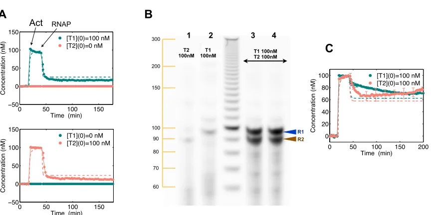
2.3.1.2 Experimental results

We expect the feedback scheme to downregulate the production of either RNA species when in excess

with respect to the other. For instance, if the concentration of [T1·A1] is twice the concentration of [T2·A2], the concentration of R1produced will clearly exceed that of R2. If the feedback scheme is working correctly, we expect to notice a decrease in the percentage of template [T1·A1]. We can easily verify this hypothesis by labeling the 5’ end of the non-template strand of the genelets

with different fluorescent dyes, and by labeling the corresponding activator strand with a quencher

(35)

templates will be quenched. For instance, when A1is stripped off T1, the T1fluorescence signal will

increase. For convenience, the fluorescence traces will be processed to map the measured signal to

the corresponding active genelet concentrations. In all the fluorescence traces shown here, the total

amount of activators is stoichiometric to the total amount of templates: [Atot

i ] = [Ttoti ].

Figure 2.12 A shows the behavior of the two genelets in isolation: we can verify that each

genelet self-inhibits after the enzymes are added. (For details on the data normalization procedure,

refer to Section 2.3.1.3.) The concentration of RNA present in solution can be measured through gel

electrophoresis, as shown in Figure 2.12 B: lanes 1 and 2 show that transcription is effectively absent.

When the two genelets are present in solution in stoichiometric amount, their RNA outputs bind

quickly to form a double-stranded complex, and therefore the feedback loops become a secondary

reaction (by design thermodynamically less favorable than the R1·R2complex formation). As shown in Figure 2.12 C, the two genelets only moderately self-repress. The total RNA concentration in

solution is high, as shown in the denaturing gel in Figure 2.12 B, lanes 3 and 4. A discussion on the

accuracy of the gel data is in Section 2.3.1.3.

When the templates [Ttot

1 ] and [Ttot2 ] are in different ratios, the system behavior is shown in

Figure 2.13 A. We can plot the resulting initial active template ratio (which corresponds to the total

template ratio) versus the steady-state one: we find that the system behaves symmetrically and the

steady-state ratio is close to one across all the initial ratios. Therefore, given open loop transcription

rates that differ across a factor of 1–3, these results suggest that the system robustly matches the

flux of R1 and R2. If the concentration of [Ttoti ] and [A tot

i ] is changed over time, the steady-state

concentration of active genelets adjusts as shown in Figure 2.14 A and B. Samples from this set of

experiments were analyzed using a denaturing gel: the results are shown in Figure 2.14 C and D

(corresponding to the traces in Figure 2.14 A and B, respectively) and show the total RNA amount

in solution and that [Rtot

1 ]≈[Rtot2 ], as desired (Figure 2.14 E and F).

The data in Figure 2.13 A were fitted using MATLAB, restricting the search algorithm to optimize

a subset of parameters that are shown in Table 2.2. This subset of parameters was chosen to assess

whether varying the branch migration rates and the enzyme speeds could satisfactorily explain the

data collected. Such parameters were used to numerically compute equations (2.12), generating the

simulated time traces shown in dashed lines in Figures 2.12 and 2.13. The fitted parameters differ

from the initially postulated parameters: in particular, the binding rates for activation, inhibition,

and output formation are much faster than what initially was assumed (Table 2.1); in particular,

the fitted output formation rate is too high and not physically acceptable. Clearly, the current fits

may be improved by extending the parameter space; this will be part of the future work on this

(36)

0 50 100 150 −50

0 50 100 150

Concentration (nM)

Time (min) [T1](0)=100 nM [T2](0)=0 nM

0 50 100 150

−50 0 50 100 150

Concentration (nM)

Time (min) [T1](0)=0 nM [T2](0)=100 nM

0 50 100 150 200

0 20 40 60 80 100

Concentration (nM)

Time (min) [T1](0)=100 nM [T2](0)=100 nM T1 100nM

T2 100nM T1

100nM T2 100nM

100 150 200 300

90

80

70

60

A

B

C

R1

R2

1 2 3 4

[image:36.612.110.542.95.311.2]

Act RNAP

Figure 2.12: A. Experimental data showing the isolated active genelet concentrations as a function of time: the self-inhibition reaction turns the switches off, and the RNA concentration in solution is negligible, as verified in the gel electrophoresis data in panel B, lanes 1 and 2 (samples taken at steady-state after 2 h). Dashed lines represent numerical trajectories of equations (2.12), using the fitted parameters in Table 2.2. B. Denaturing gel image: lanes 1 and 2 show that the switches in isolation self-inhibit and no significant transcription is measured. Lanes 3 and 4 show the total RNA amount in samples from the experiment shown at panel C, taken at steady-state after 2 h. When the genelets are in stoichiometric amount, their flow rates are already balanced and there is only a moderate self-inhibition.

Table 2.2: Fitted Parameters for (2.12)

.

Units: [1/M/s] Units: [1/s]

kT_iA_i = 2.9·105 kcatON_ii= 0.06

kTiAiRi= 5·10

5

kcatHii=.09

kAiRi = 5·10

4

kcatHji=.09

kRiTj = 1·10

3

kRiRj = 2·10

[image:36.612.249.398.581.676.2]

(37)

0 50 100 150 200 0 20 40 60 80 100 Concentration (nM)

Time (min) [T1](0)=50 nM [T2](0)=100 nM

0 50 100 150 200 0 20 40 60 80 100 Concentration (nM)

Time (min) [T1](0)=100 nM [T2](0)=50 nM

0 50 100 150 200

0 50 100 150 200 Concentration (nM)

Time (min) [T1](0)=100 nM [T2](0)=200 nM

0 50 100 150 200

0 50 100 150 200 Concentration (nM)

Time (min) [T1](0)=200 nM [T2](0)=100 nM

0 50 100 150 200 0

100 200 300

Concentration (nM)

Time (min) [T1](0)=100 nM [T2](0)=300 nM

0 50 100 150 200

0 100 200 300

Concentration (nM)

Time (min) [T1](0)=300 nM [T2](0)=100 nM

A

B

0 1 2 3 4

Final ratio of active genelets

Initial ratio of active genelets

Numerical Model No feedback

Data: T1 Varied, T2 Fixed Data: T2 Varied, T1 Fixed

0 100 200 300

0 20 40 60 80 100 Concentration (nM)

Time (min) [T1](0)=100 nM [T2](0)=100 nM Act RNAP

Analysis, Design, and in vitro Implementation of Robust Biochemical Networks