Quantitative Methods for Optimizing the Allocation of Police Resources

Journal of Criminal Law and Criminology

Volume 57 | Issue 2

Article 11

1966

Quantitative Methods for Optimizing the

Allocation of Police Resources

Robert P. Shumate

Richard F. Crowther

Follow this and additional works at:

https://scholarlycommons.law.northwestern.edu/jclc

Part of the

Criminal Law Commons

,

Criminology Commons

, and the

Criminology and Criminal

Justice Commons

This Criminology is brought to you for free and open access by Northwestern University School of Law Scholarly Commons. It has been accepted for inclusion in Journal of Criminal Law and Criminology by an authorized editor of Northwestern University School of Law Scholarly Commons.

Recommended Citation

THE JOURNAL OF CIMINAL LAW, CRIIINOLOGY AND POLICE SCIENCE Copyright 0 1966 by Northwestern University School of Law

VoL 57, No. 2

Printed in U.S.A.

QUANTITATIVE METHODS FOR OPTIMIZING THE ALLOCATION OF

POLICE RESOURCES

ROBERT P. SHUMATE AND RICHARD F. CROWTHER

Robert P. Shumate is President of Systems Science Corporation, Bloomington, Indiana. He is a former faculty member of the Department of Police Administration at Indiana University, and while there served as Director of the Police Services Group.

Richard F. Crowther is an Assistant Professor in the Department of Police Administration at In-diana University. Currently he is on a leave of absence and working with Systems Science Corpora-tion to implement a resource allocaCorpora-tion model for the St. Louis Police Department-EDITOR.

The chief executive of even a moderate sized police department is faced daily with a multitude of complex problems requiring decisions. He must strive in the face of apparently conflicting data, within a limited time, to make decisions on a ra-tional basis. Many problems, however, require an assessment of facts and a reconciliation of inter-relationships on a scale far greater than intuitive judgment alone can assimilate. Within this con-text the need for quantitative methods of analyz-ing administrative problems is becomanalyz-ing more obvious to the contemporary police administrator.

The size and complexity of today's enforcement problems result from many factors. Historically there has been a continual growth in police service due to urbanization, increase in the number of laws and regulations to be enforced, and the break-down of traditional morality. In addition, police work loads have increased because of new duties, for example those varied duties associated with road traffic.

Police departments have responded in several ways to these changes. There have been increases in total man power, application of new methods of transportation and communications, use of new techniques for record keeping, introduction of new concepts of organization, and adapting many specialized tools and techniques from scientific fields. At the same time the effectiveness of indi-vidual police officers has been improved through selection, training, and supervision. In a large measure the increased demand for police service has been met by greater productivity, rather than by simply increasing the size of forces.

The area which has received its share of atten-tion in recent years is the allocaatten-tion of police resources. Real success in developing workable methods has been elusive. Successful quantitative methods for resource allocation in industry

gener-ally assumes the existence of a success criteria, such as higher profits or reduced costs. In the police field the first problem is to find a compa-rable value scale. Unfortunately, law enforcement does not have a clearly defined "success criteria" causing difficulty in utilizing quantitative tech-niques for rational decision making.

From a formal standpoint the allocation of police resources can be viewed as two problems. The first involves the total amount of police time required to perform tasks. The second concerns the problem of preventative patrol activity and the question of how police units should be de-ployed. Of the two the former is easier to solve within some formal system because basic assump-tions are much easier to develop and verify. Com-pare for example the problem of determining the average length of time a police unit takes to per-form a task associated with the given class of events, such as street crimes, with that of estimat-ing the preventative effect of a police unit movestimat-ing from point to point within a beat.

An essential feature of the first or general police manpower assignment problem is that demands for services occur irregularly in time. In addition, the police agency has only limited control over the manner in which demands for services occur. Once the functions of a police agency have been defined, the agency must accept the pattern of demands as they occur. Collectively, these demands constitute a fact to which the agency must adjust.

R. P. SHUMATE AND R. F. CROWTHER

Therefore, while queueing theory will be freely used, the mathematical content will be minimized. The two terms "task" and "event" will be used in a special way, throughout this discussion. Within a city or other political subdivision, events occur which for one reason or another (legal, policy, political) the police have assumed a re-sponsibility. These may be traditional crimes such as homicides, robberies or assaults. They also include such activities as providing emergency care for sick people, caring for lost children or arbitrat-ing family quarrels. Associated with each such event that occurs is a task characterized by the fact that it requires time to perform, skills on the part of the performer, and usually some type of equipment. Thus, when a homicide or a family quarrel occurs, the police have a task to perform which will absorb some portion of the total police resources.

The frequency with which tasks occur multiplied by the length of time required to complete a single task determines the total amount of police time required during any given time period. For the sake of discussion, assume a situation where for a twenty-four hour time period 42 events occur. The average time required to perform a single task is 25 minutes making it obvious that a total of 1050 minutes of police time will be required to service tasks that occur during the twenty-four hour period. If only these factors are considered, it appears that three police units, one for each eight hour period, will be sufficient to perform all tasks. However, as will be noted later, the distribution of task origination times has an important effect on manpower allocation.

At this point it is necessary to digress from the main topic for the purpose of defining the notation that will be used. As the problem of manpower allocation is developed, it will be necessary to illustrate various concepts by means of diagrams. To aid in clarity and interpretation, a standard notation will be used throughout which will be defined as follows:

(T) will be used to designate an arbitrary point in time such that subsequent times may be designated T + 1, T + 2,-.-T + N where the integer refers to increments of one minute; thus, T + 10 would be read, "The arbitrary starting time plus ten minutes."

(E) will be used to designate an event that generates a police task with the subscripts E1, E2, --- E. defining n classes of events.

(P) will be used to represent a police unit and will use lower case alphabetic subscripts P., Pb, "'" P. to specify particular police units.

The symbol (--) will be used to mean "Occurs at"

such that the expression E1 - T would read, "A type 1 event occurs at time T".

As a means of quickly referring to a given block, both the columns and the rows will be numbered 1, 2, 3, --- n. Thus, each block has a unique ad-dress specified by two numbers. A reference to block 1, 1 means that the block in the first row and the first column. A rule will be adopted that it takes one minute for a police unit to travel from a point on one block to a corresponding point on any adjacent block. This rule will be extended in such a manner that police units may move only along rows or columns and cannot move diagonally. Complete familiarity with the notation will facili-tate the readers subsequent understanding of the material.

1 2 3

Pa--T+4

E₃-T+42 E2-tT.19

2

-Pa-T43 Pa-.-T+22

3

P

_T

FIGmR 1

POLICE RESOURCE ALLOCATION

and completes the task at T + 42. At T + 42 a new task is generated at 2,2 with the police unit arriving at T + 43. At T + 68 the police unit will have completed the task and be ready for either patrol or the performance of a new task.

This is an illustration of the kind of distribution of task starting times which is the most efficient from a manpower allocation standpoint. In this

case, events occur such that as soon as the police unit completes one task, he moves directly to the next. Unfortunately, police tasks are rarely gen-erated in this fashion over any extended period of time. To illustrate the problems normally asso-ciated with the distribution of police tasks, con-sider Figure 2.

1 2 3

E2"-*T

1

Pa-T+4

2 E₃-T+4 E₁--T+5

3 Pa -T

FiGuRE 2

Beginning at some time T, Pa occupies bloc, 3,3. At T an event E2 is generated at 1,1. At T + 4,

Pa arrives to perform the task which will be

com-pleted at T + 19. Meanwhile, at T + 4 two new tasks have been generated at 2,2 and 1,3. A police unit can by definition perform only one task at a time. Thus the two tasks originating at T + 4 cannot be performed by Pa for at least 17 minutes (the time to complete the task at 1,1 plus travel time) and even then one of the two tasks will have to wait until the other has been per-formed before it can be completed. To make the situation more complex, at T + 5, a fourth event (E,) is generated at 2,3.

Thus, by comparing the two problems just illustrated, one can see that answering the ques-tion, "How many units do we need?" is not always easy. The same total amount of police time is re-quired in both examples but beyond this there is a

great difference. In one case the police time is needed at a single point in time, in the other it is spread out over time. In the second illustration there are several tasks waiting for service. It is customary to speak of these waiting tasks as being in queue.

Considerations such as these form the basis for a whole class of problems directly related to the question of how many patrol units are required to service an area. The answer to this question in the first example is that a single unit will satisfactorily perform all police tasks with only a minimum of delay. In the second example, applying the same criteria, it would be necessary to have four police units available. But consider the further possi-bility in the second example that after the fourth task has been performed, no other tasks are generated for several hours. What then is the justification for having four units idle for several hours when, to begin with, it is likely that the police department has only limited resources in terms of manpower and equipment? When the problem is stated in these terms it becomes a queueing problem.

There are many examples of familiar social processes that are essentially queueing problems. For instance the total capacity of public trans-portation system in a metropolitan area is deter-mined in part by the average workload and in part by the average rush-hour workload. The result is, of course, that in rush hour the effective capacity of the system is strained. Another example, is a communication system such as the telephone company. The scale of these systems are set so that most of the time there is excess capacity. During those times when a great deal of service is required, the systems become overloaded. There are other more homely examples. Anyone who has waited to get into the bathroom is suffering from the interactions of an irregular demand for service on a fixed capacity facility.

Essentially, a queueing situation occurs when a facility with a limited capacity for providing service is required at irregular intervals to handle a load in excess of the capacity. If there is no reason to avoid delays, then there is in effect no real queueing problem. If on the average the capacity to perform tasks is greater than the average rate at which events occur, from time to time the servers will succeed in catching up with the work load.

Whenever there is some cost associated with delay, however, problems arise. If the waiting time

R. P. SHUMATE AND R. F. CROWTHER

UNIFORM ARRIVAL TIME IN MINUTES

0 10 1 1 i 0 1 0 0 10 10 0 0 10 0 10 0 0 10 10 10

I i I I I I I I I I I I I 1 I I I I I I I

Fiouax 3

produced by delays is to be reduced, the capacity of the service mechanism must be increased. When this is done, however, the amount of idle time for the facility also increases. In the case of a police facility, the extra capacity must be paid for no matter in what manner it is used. In general, doubling the police manpower would roughly double the cost of the service. Two major com-ponents of the return from the increase in service capacity are the reduction in the amount of wait-ing time, and the return for such other activities as the manpower can be used for when on duty but not servicing a call. It is evident that eventu-ally the costs and returns from the scale of opera-tions should somehow balance. It is also evident that this is a problem which is not easy to solve. The first question that must be answered is whether the conditions that produced the situa-tion in Figure 2 are likely to occur frequently or whether they can be expected to occur only on occasion. If the latter is the case, it may for eco-nomic reason, be necessary to occasionally delay even important tasks. On the other hand, if such a situation is likely to occur frequently, steps must be taken to provide manpower to meet the demands.

We will consider one possible way of dealing with this type of problem. To do so, conditions will be simplified as far as possible to permit the reader with a limited mathematical background to follow the reasoning involved and to see the concepts utilized against a background of familiar terms.

For purposes of illustration, a modest size beat, 9 blocks square, will be used. The problem will be limited to consideration of the hours between 12 noon and 2 p.m. assuming that in the course of one year 800 events that require police attention will occur during these two hours. The problem to be solved may be posed as a question. If one police unit is assigned to this beat, how often will it be necessary to delay servicing events because the police unit is already engaged in performing a prior task?

A convenient starting point is a consideration of the manner and rate in which events will occur. Considering first the rate at which events will occur, the first task is to select some appropriate time interval to work with. Since the time re-quired to perform a police task is usually measured in minutes, a time interval of one minute will be used. During a one year period there will be 43,800 minutes during the two hour period we are con-cerned with. The average rate per minute at which events occur is 800/43,800 = .018 events per minute. While it may seem odd to think of a frac-tion of an event, it will become evident that it is a useful basis for expressing the rate at which events occur.

It will prove useful to view all events as having arrival times. Arrival time means the time that an event occurs. Thus, if an event E occurs at 12:13 p.m., the event's arrival time is 12:13 p.m. The time between the arrival of successive events will be referred to as interarrival gap. Before useful conclusions can be reached concerning the conse-quence of assigning one police unit to our hypo-thetical beat, it is necessary to know something about the distribution of arrival times and in particular interarrival gaps. The concept of dis-tributions may be an unfamiliar one, so we will digress for a moment to clarify the conceptat least in regard to arrival times.

Figure 3 illustrates one way in which events might occur. Note that in this case events occur at evenly spaced increments of time to produce uniform interarrival gaps of 5 minutes. In this case, the variation of interarrival gaps is 0. In other words, the time between arrivals are all exactly 5 minutes apart and no other interval is observed. A graph constructed to portray the frequency with which various interarrival gaps occurred, would look like Figure 4.

POLICE RESOURCE ALLOCATION

0 1 2 3 4 5 6 7 8 9 10 FIGURE 4

between events, therefore, the average is 120/24 =

5. The distribution of times about the mean, or

variance as it is often referred to is 0 which can be verified by direct observation as well as by calcula-tion. The two concepts of means and variance (distribution) will become important as formal methods for solving the manpower requirement problem are developed.

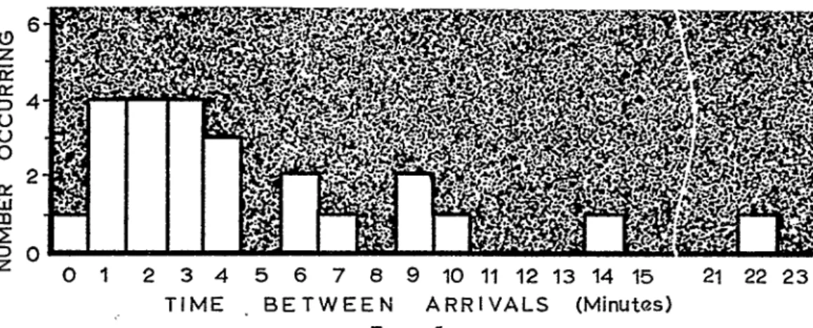
It is rare that we find natural phenomena occur-ring at fixed intervals of time and certainly it is not the case where police tasks are concerned. Figure 5 portrays the manner in which events that the police are concerned with usually occur in time. Consider both the similarities and differences be-tween the two illustrations of arrival times. Note that both have the same average, 5 minutes. How-ever, the distribution of interarrival gaps differ widely which can be verified by comparing Figures 3 and 5. In the case of uniform interarrival gaps, the intervals are all alike, whereas in the

non-uni-6

z

0 .~ ...

form group, there are interarrival gaps ranging from 0 to 22 minutes.

Examination of the arrival times of many thou-sands of events that generate police tasks have shown that the interarrival gaps are distributed in a manner similar to that shown in Figure 6. The arrival time distribution about the average fits quite closely to a "Poisson" distribution curve. Drawn in graph form, this distribution looks like

Figure 7.

Since a limited number of interarrival gaps were used in the example, the distribution shown in Figure 6 does not dearly show the shape of the "Poisson" curve. If observations from a large number of interarrival gaps, for example 500, were used, the distribution would look something like the one shown in Figure 7. Here it is possible to see quite clearly the shape of the curve from the frequency histogram. The "Poisson" distribution has been widely used in the formal analysis of somewhat similar problems. While in many cases it is not an exact representation of the way nature generates the events, it so closely approximates what is actually observed that it is of great utility. Practical applications of this distribution have occurred in problems involving radioactive decay, motor vehicle traffic accidents, telephone system capacity, and customer service problems in many fields.

One of the useful things about the "Poisson" distribution is that many of its properties can be expressed mathematically. If we are willing to accept the premise that interarrival gaps for police events will group about the mean this way these properties can be used to compute probabilities relating to future event arrival times.

Since the question we seek to answer is, "What

fl Afl ~44 Afi 4.. .44 Ar t94 fin fin

TIME

BETWEEN

ARRIVALS

(Minutes)

FIG RE 5

400

350

300

(.9

z

" 250

C)

o

200

ry

w

ED 150

100

50

0

80-

70-60

50

40

30

20

10

0d

01 23456 7 8 9 10 11 12 1314 15 161718 19 202122 2324

FiGuRE 7

202

3 4 5 6 7 8 9 10 11 12 13

TIME BETWEEN ARRIVALS

FIGURE 6

POLICE RESOURCE ALLOCATION

are the chances that events will happen faster than the police unit assigned to our hypothetical beat can service them?", it is necessary to know something about the length of time it takes a police unit to service a given event. For the sake of illustration, assume that it requires 25 minutes for the police unit to service one event. For the time being, travel time required to get to the scene will

be ignored. A practical restriction that a police unit can service only one event at a time will also be observed.

It was pointed out earlier that one of the useful things about the "Poisson" distribution was that certain of its properties could be expressed mathe-matically. Advantage can now be taken of this property of the "Poisson" distribution to compute the probability of 0, 1, 2 and 3 events occurring during the next minute. This can be done by

solv-ing the following equation. The terms to the left of the equal sign may be read as, "the probability

P(nIx) = ex

(P) of some number of events (n) where the average rate per unit of time (x) is known". Thus, to ask the question, "What is the probability of one event occurring during the next minute?", the actual values can be substituted for the symbols:

P(1 1.018) which is read, the probability of one

event occurring during the next minute where the average number of events occurring in a minute is .018. To the right of the equal sign, e is a con-stant whose value is approximately 2.7183, x is the average rate of occurrence per unit of time, and n in both the numerator and denominator refers to the number of events that we want to evaluate for. The term n! is read n factorial. To understand what factorial means, consider 3! which is 1 X 2 X 3 = 6, and 4! which is 1X 2X 3X 4 = 24. By definition 0! = 1.

From a computational standpoint, evaluating

e x in the formula is the most difficult. There are several ways to approach the problem, but a method which seems to have the greatest intuitive appeal and which is straightforward, if somewhat tedious, is to use the series:

x

x

+

x+

2! 3! 4! 5!

This series has the property that the error in estimating the value of e will be no greater than

the last term in the summation.

Let us proceed to solve our problem by first

evaluating e- for our problem where the values to be solved are:

.0003 .000006

e- = e-0 18 = 1 -. 018

+-

2 6

Note that only three terms in the series were eval-uated since to go further would be to seek accu-racy that would be of little practical use.

Substituting the value for e-x in the original equation, the probability of 0, 1, 2, or n events occurring in one minute can be determined. Thus:

For zero events during the next minute:

.982

X 1

P(0 1.018) =

1

.982

For one event during the next minute:

= 982 X .018

018

P(1 1.018) - 1 _.1

For two events during the next minute:

P(21.018) = 982 1 +.00016

and for three events:

P(3 1.018) .982 x .01836 +-.00000097

Several statements concerning the occurrence of future events can now be made. Selecting a start-ing time at random, the probability that no event will take place during the next minute is .982 which is another way of saying that the odds are about one hundred to one that nothing will occur during the next minute. The probability of 1, 2, and 3 events occurring are, respectively, .018, .00016, and .00000097. Thus, for the problem selected, the chances of even one event occurring during the next 1 minute is a slim one.

The method can now be used to solve a more practical problem. If the police unit has just begun the performance of a task at time (T), what is the likelihood that other tasks will occur before the first task can be completed? The average rate at which events occur has already been deter-mined to be .018 per minute. It follows from this that the average rate for 2 minutes is .018 X 2 or .036, for three minutes, ,018 X 3 or .054, and for 25 minutes (the length of time required to perform a task) .018 X 25 = .45. Using the method pre-viously outlined, first evaluate e- as follows:

.452 .451 .454

e-'45 =

1

-.45+

--

+-2 6 24

=1 -. 45 +.101 --. 0152 +.002 = .638

R. P. SHUMATE AND R. F. CROWTHER

Then substituting in:

P(n I x) = eXn

Ve obtain for different values of P:

.638 x .450

P(O01.45)- =

3

638 x .451

P(l1.45) 1 .287

.638 x .452 P(2

1.45).-

.638 X .451

P(31.45)--

6

It is now possible to make some useful observa-tions about what is likely to occur if only one police unit is available in the beat during the two hours under consideration. A matter of interest is the frequency with which it will be necessary to delay servicing tasks and the length of the delays.

It is impossible to predict exactly how long any individual task will have to be delayed since the second task may occur any time during the twenty-five minutes. However, since some of the time the second task will occur during the first minute, sometimes during the second minute, etc., the average length of the delay will be about

Y2 the total task time or 12 minutes.

The first task in queue will average 12Y- minutes of waiting time before it can be serviced. What about the second task? If a rule is adopted that tasks are performed in the order in which they occur, the second task must wait the original 12Y2 minutes plus the time it takes to perform the first task in the queue which is 25 minutes. In fact, a general formula for computing the delay for any number of events is: d = E(n - 1) + ( 2)E where E is the time required to service a single event and N is the number of events for which we desire to determine the delay. Thus on these occasions where two events occur, the delay time will total 37 2 minutes. The delay associated with a third event occurring while the first event is being serviced can thus be calculated as: 25 X 2 + 12 = 62 2 minutes. Returning to the original calculations, it was determined that the probability of a second event occurring while the first was still being serviced is .287. Another way of expressing this is to say that 28.7% of the events that occur will have to be delayed while the

patrol unit finishes servicing the event he is already working on. Since 800 events are expected to occur during the year, 28.7% or 230 times a year this situation will occur in which service will have to be delayed 12 2 minutes. Similar calculations

can be made to determine how often longer delays will be encountered. In brief, the results are: 51 times per year an event will have to wait 372 minutes for service and about 8 times per year an event will have to wait 62 minutes for service.

Thus, once the probability of 1 or more addi-tional event occurring before the first can be serviced has been calculated, we have a measure of the frequency and size of the delays that will be encountered.

Until now we have talked about the probability of a second, third, or n event taking place before the police unit finished servicing the original event. This way of looking at events is an excellent way of illustrating concepts and the probabilities calculated are correct as far as they go. However, while the police unit is servicing the events already waiting the probability of additional events taking place increases. One way of dealing with this problem and also providing additional information is to view events in a slightly different manner.

It is possible to rephrase the question to ask, "What is the probability of having one or more events already waiting in queue for service when a random event occurs?" This is almost like revers-ing our previous question. As concepts are de-veloped more fully, thinking in terms of the probability of having a specified number of events waiting in queue will prove extremely useful. For example, a formula for calculating the probability of finding 1, 2, 3, --- n events in queue when any event selected at random occurs is available. From these calculations other useful information can be obtained such as the average delay time and the effect of adding additional police units to service events.

Before presenting this formula there is a statistic that is important in queueing theory that should be considered. The calculations required for the type of problem being considered here need not depend on the unit of time used. If, for instance, it is more convenient to state the time interval as a decimal fraction of an hour the number of events may be expressed as the number of events per fraction of an hour used. The average service time should be quoted in the same time unit. The results in this case would be stated in decimal frac-tions of an hour.

POLICE RESOURC

A system of time units which can be used to considerable advantage utilizes the relationship between the interarrival gap and the service time. Either the average interarrival gap or the average time required to service an event can be called one unit of time. Whichever unit is selected, the other is expressed in terms of the first. For example, if the average interarrival gap is called one unit of time, then the average service time is expressed in p time units. Thus, the statistic p represents the ratio between the average interarrival gap and the average time required to service an event.

P

Where [ is the average service time and X is the average interarrival gap.

The statistic p is important both to simplify calculations and because it is a measure of con-siderable value in its own right. In any situation if p is less than one sooner or later every event that occurs will be serviced. If, on the other band, p is equal to or greater than one, tasks will occur faster than they can be performed and the queue of tasks will grow indefinitely.

The formula for calculating the probability of n events being in queue awaiting service when any event occurs is:

P0 =1- p

Pi

pn= (I - )[

n-i (-pi)n-i-lePil

i=0 (n - i-i )!

The calculation of probabilities for various values of n using the above formula would be a formi-dable task if the calculations were performed by hand. It poses no problem, however, for a digital computer. The problem used to illustrate the con-cepts so far assumes fixed service time of 25 min-utes and an average interarrival gap of 54.7

25

P =

5

minutes. Thus, a table for values of n from 0 to 8 for a p of .455 is provided in Table 1. Also shown are the probabilities of finding n or less and n or more events in queue. The probabilities presented in the table differ slightly from those calculated previously for two reasons. This formula is a more

T ALLOCATION 205

precise method and it takes into consideration the fact that while tasks are waiting in queue the probability of additional events occurring in-creases.

TABLE 1

Number Delay in Probability Probability Probability of Events Minutes of Eexatly

of~~~ Eventss Mfue

~E

0 0 .5450 .5450 1.000

1 12.5 .3140 .8590 .4550

2 37.5 .1041 .9631 .1410 3 62.5 .0278 .9909 .0369

4 87.5 .0069 .9978 .0091

5 112.5 .0017 .9995 .0022

6 137.5 .0004 .9999 .0005

7 162.5 .0001 1.0000 .0001 8 187.5 .0000 1.0000 .0000 Once the probability of n events being in queue is known (Col. 3, Table 1) the probability of en-countering a delay of n minutes can quickly be determined utilizing concepts already discussed. The first event in queue will result in an average delay of 122 minutes and subsequent events that enter the queue will create a 25 minute delay under the assumptions in our problem. Thus, for five events in queue, d = 100 + 12.5 = 112.5.

These calculations have been made and are pre-sented in Col. 2 of Table 1. Looking up the proba-bility of 5 events being in queue in Col. 3, Table 1, we find the probability of encountering a delay of

112 minutes is .0017.

Normally such a question is posed in the form, "What is the probability of encountering a delay of 112 minutes or more?" This question can be answered by turning to Col. 4, Table 1, and ex-amining the probability for n = 5. This shows that the probability of a delay of 112 minutes or more is .0022 which means that about 2 times out of a thousand events a delay at least this long or longer will occur. Thus, by using a table of p values from .00 to .99, many useful questions can be answered concerning the likelihood of delays of varying magnitude occurring.

R. P. SHUMATE AND R. F. CROWTHER

earlier, the assumption was made that for every event the police unit required exactly twenty-five minutes to perform the task. Obviously this is not the way task performance times behave under actual conditions and if the principles illustrated so far are to be applied to real problems a way must be found to deal with variable task times. Actually the time required to service an event will vary from one event to another. In other words, the service times will have a distribution just as interarrival gaps do.

A measure of the amount of delay that can be expected for a given beat is the average delay time. The average delay time for any value of p where a non-fixed service time is assumed can be deter-mined by the formula:

E(d) =- x p +p'(1 +d

The symbol c is the partial coefficient of variation which is the ratio of average service time (1i) to the standard deviation (a/lz). The symbol p has been previously discussed and x is the number of events occurring per minute.

Thus, if the assumption is made that the service time used in the problem represents an average of 25 minutes with a standard deviation of 5, then

c= 25)2 = .04 The average delay

[4 .207(1 +

.04)1]

E(d) = 54.7

.455

is 35.6 minutes. The average delay time has the disadvantage that it does not give specific in-formation about the chances of encountering delay above a certain level but it does give some idea of the magnitude of the delay likely to be encountered. It also provides a means for dealing

successfully with non-fixed service times which become important in any real problem.

While a good many problems can be solved by quantitative methods, it would be a mistake to assume that quantitative methods can be applied indiscriminately to police problems with the expectation that they will invariably produce improved decision making. To so assume would be to confuse technique with the substantive process of administrative decision making. After all, the goals and values which are at the heart of all police problems are human goals and values. In this realm any method or technique must be regarded as a tool controlled by and subservient to those who use it.

Consider the problem that has been used as an illustration. The decision, whether to utilize one or two units to service calls originating on the beat, will in the end be value oriented, involving an assessment of citizen reaction, resources available and the current political climate.

In the long run the administrators will tend to be able to make more effective decisions if he understands and uses analytic techniques as opposed to a completely intuitive approach. Through analysis he has quantitative information available upon which to base decisions. The out-come of assigning any number of units to the beat can be assessed in terms of the delays likely to be encountered and the excess time that will be available on the other hand. He is in a better position to relate value oriented factors to the quantitative aspects such as the cost of resource and the level of service being furnished.

The preceding discussion has explored some concepts by which quantitative techniques can be applied to a particular type of police problem. The problem used as an illustration was simpli-fied to demonstrate method. However, the same techniques can be extended to provide optimum solutions for extremely complex problems in-volving a large number of beats, borrowing from other beats, and the assignment of priorities t6

different types of events.