A RULE-BASED PREDICTION METHOD FOR DEFECT
DETECTION IN SOFTWARE SYSTEM
1
B. DHANALAXMI, 2Dr.G.APPA RAO NAIDU, 3Dr.K. ANURADHA
1
Associate Professor, Department of Information Technology, Institute of Aeronautical Engineering, Hyderabad, Telangana, India
2
Department of CSE, JBIET, Moinabad, Hyderabad, Telangana, India
3
Department of CSE, GRIET, Hyderabad, Telangana, India
E-mail: [email protected], [email protected], [email protected]
ABSTRACT
Software is a complex object that consists of different modules with changing degrees of defect occurrence. By efficiently and appropriate predicting the frequency of defects in software, software project managers can better utilize their workforce, cost and time to obtain better quality assurance. This paper proposes a rule-based prediction (RBP) method for defect detection and for planing the better maintenance strategy, which can support in the forecast a defective or non-defective software module before it can deploy for any software project. The RBP extends the Ripple-down rule (RDR) classifier method to construct an effective rule-basedmodel for accurately classifying the software defects. The method will enhance the software defect prediction so that software testers can spend more time in testing those components which are expected to contain errors. The experiment evaluation is performed over a software repository datasets and the obtained results showa satisfactory improvement.
Keywords:Defect Detection, Rule-based Prediction, RDR Classification, Software system
1. INTRODUCTION
The defect prevention method does not always prevent defects in the application below test because the application is so complex and impracticable to identify all the errors or faults. The defect detection technology complements the defect prevention effort and uses both methods together to enhance the likelihood that the test team will achieve the identified test objectives and goals. The presence of "defect prevention strategies" not simply reflects anelevated level of test field maturity, but also represents the most cost-effective expenditure associated with overall testing efforts. A variety of methods, tools, techniques and methods to prevent defects are proposed, but they all seem to be insufficient n accurate prediction. More work is still to be adopted to prevent defects in terms of technology and the schemes that are used.
In the case of errors detected in the development lifecycle, requirements specifications it can be prevented errors from migrating from design and design to code. Defect prevention is critical to the quality of the organization. The main purpose of quality costs is not to decrease costs but to provide
costs in appropriate investments. It should not be delighted as a waste of time while stipulating deep participation. Instead, it should consider saving time, money, and resources it needs. It can save as many reworks as it needs when defects appear in the final or post-delivery period. At every stage of the software lifecycle, defect prevention should be introduced to prevent failures early, take corrective action to eliminate them and avoid their recurrence. A software defect prediction framework is a system that can predict whether a given software module is defective. Typically, software failure prediction models are trained utilizing software measures and fault data composed from earlier developed software releases or related projects. Models can be applied to program modules with unknown defect data.
according to defects, one of the important features of the software. A variety of data mining procedures such as "Decision Tree", "Bayesian Belief Network" (BBN), "Artificial Neural Network" (ANN), "SVM", and "clustering" are a few of the techniques commonly used to predict software defects. One of the important and effective research in the areas of software engineering is software defect prediction. Defects imperfection prediction artifacts provide a listing of source code defects so that QA team can successfully allocate insufficient resources in confirming the software by additional work on source code where defects occur frequently. As software projects grow in a large amount, the defect analytics technology participatesin an important character in keep up of the design and reduce time-to-market plays with reliable software products. Even the measurement of defect analysis and existing models cannot provide good predictive performance generally. Because every organization tries to keep this data confidential, it cannot publish data sets that can be used in experiments. One of the most commonly available data sets includes the MDP and PROMISE repositories provided by NASA. In this paper, we propose a "rule-based prediction" (RBP) method for efficient defect prediction in software systems. The most important purpose of RBP is to build an effective rule-based model to accurately classify software defects. We also use NASA repository data sets to evaluate proposals.
The following paper is categorized as Section-2 discusses the related works, Section-3 discusses the proposed rule-based prediction method in detail, Section-4 presents the experiment evaluation utilizing the datasets and section-5 discusses the conclusion of the paper.
2. RELATED WORKS
Software defect prevention proposals are mainly based on tools, techniques, methods and standards [11], [17]. This is one of the most active areas of research in software engineering, [9], [21], [10], [17], [19], [15]. Because the defect prediction model provides a list of buggy software artifacts, QA teams can efficiently assign limited resources to test and investigate software products [10], [21], [15].
A. Needs of Defect Prediction
Defect analysis at the early stage reduces time [6], cost, cost, and resources essential. Knowledge of
entering faults and process can prevent defects. The study of this knowledge will improve quality and analyze the root cause of defects can prevent the occurrence of defects. Analysis of the main reasons may take two types: "logical analysis" and "statistical analysis". Logical analysis is a human-orientedinvestigation that needs specialized knowledge in products, processes, improvement and the environment. Checks logical connection among errors (effects) and error (reason), and statistical analysis based on empirical learning of similar projects or projects generally written [18]. There are many ways to detect defects such as "inspection", "prototype", "testing" and "accuracy calibration" [7]. Formal testing is the most effective and expensive method of quality control to detect defects at an early stage of development [8], [9]. Prototyping understands the specific requirements to help eliminate some of the shortcomings in defect elimination. Testing is one of the most effectual techniques. It can escape through the early detection of defects [10] which can be detected during the test. Improve accuracy, especially in the coding phase, to determine the best way to go. Precision tuning is the most effective and economical way to create software. Defect prevention can be accomplished by automating the development process. Several tools are offered to analyze the necessity of the stage. The tools available are the requirements for being too costly. It can automate the compliance checks, but this cannot be an automatic integrity check. The tools used in this step include requirements management tools, recorder requirements tools, requirements and validation tools. Design tools include "database design tools", "application design tools", and "visual modelling tools" such as "Rational Rose". Even tools such as "code generation tools", "code testing tools", and "code coverage analysis tools" can be used to automate testing steps. Several tools such as "defect tracking tools", "configuration management tools", and "test procedure generation tools" are available at every stage of development.
B. Existing Defect Prediction Models
or statistical models, such as "BugCache" [19] have been projected.
The Figure.1 illustrates the frequency of use of the "defect prediction model" in representative defect prediction in the literature [4]. Because "statistical models" based on machine learning have been considered for anextensive time, "classification and regression models" dominate. In the proposed BugCache [29], there have been several studies examining the BugCache model as well as case studies in [12],[13],[16].
.
Figure.1: Utilization frequency of defect prediction models
Kim et al. [23] suggested a new "defect prediction model" termed as "change classification". Change classification can be directly beneficial to developers, as opposed to the common failure prediction model because the change classification model can provide immediate predictions every time a developer changes to source code files and commits to the "version control system" [21]. Though, the modified classification model is besideintense for actual use because the model consists of more than 10,000 features [16]. Turhan et al. [24] implemented a nearest neighbour filter applied (NN filter) is used to improve inter-company fault prediction performance. The basic idea behind NN filters is to accumulate related source instances in the objective instance to learn the prediction model. In other terms, if it can build a prediction model utilize a selected source instance with data characteristics similar to the target instance, the model can be better performed when predicting the target instance over the model learned to utilize all source instances. The NN filter selects 10 source illustrations for each target instance as the nearest neighbours. To evaluate the performance of inter-company fault prediction utilizing NN filters were conducted utilizing 10 proprietary data sets from NASA and SOFTLAB [24].
Most existing work on troubleshooting depends on declarative specification rules [5] [6] [7] [4]. These conditions usually determined manually identify the
main features that characterize a defect, especially utilizing a combination of quantitative (metric), structural and/or lexical information. However, in a deep scenario, the number of possible defects that can be described manually with the rules can be very large. Dimensions software typically utilized to analyze method efficiency and product software quality for the projects. Failure assessment is carried metrics software and effectively used to predict faults. For each fault, the rule represented by the metric combination requires significant remediation to find the threshold appropriate for each metric.
The software is a complex object that consists of different modules with varying degrees of defect frequency. Therefore, it is significant to predict a defective software module before it deploys a software project to plan anim proved up holding schemes. Premature knowledge of faulty software modules can facilitate it plan efficient process improvement at a reasonable time and cost. This can direct to enhanced software releases as well as higher customer fulfillment. Software modules are categorized into two categories, either defective or non-defective, and are mostly predicted utilizing a binary classification model. We take advantage of these two classes for suggestions on how to classify and evaluate data sets.
3. PROPOSED RULE-BASED PREDICTION METHOD
Figure.2: Proposed RBP Methodology
Generally, before it creates a failure prediction model and uses it for predictive purposes, it must first determine the learning scheme or learning algorithm that it will use to build the model. Therefore, the predictive performance of learning plans should be established especially for prospect data.
The framework consists of two modules:
1. Learning Phase of RBR Method 2. Defect prediction phase.
A. Learning Phase
In this framework, the proportion of splitting utilized to assess the effectiveness of everyone predictive model was first used. That is, every first data set is divided into two fractions and anidentifierlearns within 60%, and the left over is 40%.The ripple-down rule consists of a data organization and a knowledge gaining scenario. The knowledge of human experts is accumulated in the data structure. Knowledge is implied into a set of rules. In the knowledge acquisition scenario, the process of transferring the knowledge of human experts to the RBR's knowledge-based system is described.
Alogrithm-1 shows the pseudo-code view of RBR: The code consists of two nested loops. External Loop selects the class value, and the inner loop creates a rule that applies to the class. The function returns a combination "best_clause" only example in terms of covering the current class. RBR uses a simple heuristic algorithm choice of the term, which is based on the probability that a certain classification of certain attribute-value pairs. The following conditions are usually added conditions to choose the most positive and least negative pattern example. This is given by the ratio z / s, where s is the "number of examples chosen by the term", and z is a "positive number". The rule is added until the rule selects only the positive example (i.e., until z = s). RBR ensures that the rule set is complete. All examples are enforced by at least one rule and are consistent. All examples are expected to belong only to one class.
• Ripple-Down Rules
system grows and becomes more difficult due to the interplay of rules. The "ripple down rule mechanism" creates a bi-directional reliance among rules so that rule activation is simply examined in the perspective of last rule activation. If the assertion of the main regulation is true for a scrupulous personality, the conclusion about the individual is expressed if there is no dependent. However, if it is 'true', the rule and its dependents are tested in 'Where appropriate' and the original conclusion is only claimed if the premise of the institution is true to the legal object. Conversely, if a certain individual construction principal rule is false, then the conclusion is not only maintained, but if it have an "if-false" dependence, and its needy will also be tested. Thus, the "ripple-down rule" is a "binary decision tree" is different from the standard decision tree to determine the point that it uses a sophisticated branch, and it does not make exhaustive provision to settle all cases, decisions on the internal node. This disparity with the standard tree, where the entire decisions are the source node. However, the functionality of the "standard decision-tree" claims that only one decision node is active in each case. This is effortless to maintain, as it should be taken into account only the nodes of a past event if there are errors in reaching decisions.
The expansion of the ripple-down rule involves a very simple statistical decision process to create a regulation that is recursively termed in the remaining data set to produce true" and "if-false". It is a very natural in pointing rule. Figure.-3 shows the fault analysis, which offers a "statistical control algorithm" used to fit. The case in the area under consideration for the share is displayed as a rectangle off rectangle fault. The rectangle with the defect D0 is the rectangle that the Induct tries to determine the rule. If the premise of the currently proposed rule applies, it will be displayed as an outer ellipse. An internal ellipse indicates a collapsed set that applies when a supplementary article is added to the principle rules.
Figure.3: Inducing ripple-down rules
There are three stages to creating a principle rules. First, the generally frequent diagnosis in the fraction under deliberation is opted for as the object description. Second, the area is started without a clause. Third, the combination of the value of each property that has been tested is available on the best possible terms and selected according to statistical tests in detail below. Fourth, the time that the provision of such tests determined whether the rules have improved. If there is an improvement, the process can be repeated for the third step, otherwise, the product will finish ruling with the rule output.
The data construction is related to a "decision tree". Everyone node has a rule and the arrangement of this rule is "IF cond1 AND cond2 AND ... AND
condNTHEN conclusion". "Cond1"is a clause of
the 0 or 1 evaluation. For instance, if "A=1", then "is Greater (A,5)" and "average(A,">",average(B))".
Everyone node has precisely two supporting nodes, the supporting nodes are associated with the node by "ELSE" or "EXCEPT". An instance of "RDR tree" which described repeatedly is given below:
B. Defect Prediction Phase
The methodology of defect predictive phase is straightforward. It consists of an"identifiercreator" and "defect prediction". During the identifier construction phase, a learning plan is selected. Predictive variables are created with the selected learning plan and full historical data. The end result is the average of all surroundings. This shows that the assessment actually cover up all the data. Therefore, building identifiers utilizing all historical data is expected to improve the simplification capability of built identifiers. After the identifier is created, novel data is pre-processed in anequivalentmanner as historical data, and afterward the identifier built can be utilized to predict software faults with latest pre-processed data. The difficulty of "empirical prediction induction" is specified by a "universe of entities",
E, "a target predicate", Q, and a "set of possible test predicates of the form", S on entities in E, to utilize them to create a set of rules from which the intention predicate could be conditional specified the assessments of the test predicates. For the intention of the "statistical analysis", the appearances of S and Q which do not substance. One should consider S as anidentifier to select those "e" out of several separations of E for which to claim "Q(e)", and measure up to the assortment method of the regulation with that of indiscriminate identified, the enquiries to find “what is the probability that random identification of the same degree of generality would achieve the same accuracy or greater" is been shown with help of the Figure.4.
Figure.4: Defect investigation for statistical organize of empirical orientation
Lets considered "Q" be the "associated entities" in
E for which "Q(e)"contains, S be the "selected entities" in E for which "S(e)"contains, "C" be the "correct entities" in E for which both "S(e)" and "Q(e)" contain. It can represent as,
(1)
(2)
(3)
Let's the "E, Q, S" and "C" be "e, q, s" and "c" are cardinalities of correspondingly, and the probability, p for getting from E which will contain
Q at a random will be computed as,
(4)
The process of complete outlining the mechanism of enhancing RDR approach is presented in Alogrithm-2. It discusses a function "make_rdr" which takes default class attributes and training set as input to provide the new RDR rules.
the best term for each step is based on decreasing the probability that the result accomplish by the assertion is accomplish by "random identification". For "ripple-down rules", a significance decision is whether to maintain the further common rules for external ellipses or to add additional clauses that correspond to internal ellipses. An external ellipse covers additional target cases that utilize"D0" as a diagnostic, except it contains more "D7", "D8", "D9", etc., so it should be delighted as an exception in the "ripple-down rule" structure. The decision is fascinating because it does not essentially influence the accuracy of the ultimate knowledge to stand given the ability to handle exceptions. Relatively, it influences the structure in expressions of preferences for generic rules with various exclusions relatively than definite rules with only some exceptions. It affects the quantitative measures of the knowledge base, such as the number of rules and conditions concerned, but influences the structure in a way that human experts can present knowledge in a way that pertains to cognitive approaches.
4. EXPERIMENT EVALUATION
The experiments were performed utilizing algorithms implemented in the "WEKA environment" [19] utilizing NASA - Metric Data Program (MDP) Repository. Below we discuss datasets, evaluation measures, and results analysis.
A. Datasets
[image:7.612.312.525.98.209.2]The datasets are obtained from the "NASA-MDP Repository" [9] which consists of 12 datasets. Data storages contain metrics software quality attributes in data sets, as well as an indication of whether a particular set of data is "defective" or "non-defective". Each data set consists of several software units, each corresponding to many of defects and different software code static characteristics. The preprocessingunits contain additional defects seen as defective. A more comprehensive description of "code attributes" or "the origins of the MDP data sets” are available in [5]. The number of data sets utilized is"CM1, JM1, KC1, KC2, and PC1", which include" static code measures" discussed by "Halstead" and "McCabe", along with defect rates. Table-1 presents project narrative for every one of these data sets.
Table 1.Each Project Data Set Description Project Source
Code
Description
CM1 C NASA spacecraft instrument KC1 C++ Storage management for
receiving/processing ground data KC2 C++ Science data processing. No software
overlap with KC1 JM1 C Real time predictive ground system PC1 C Flight software for earth orbiting
satellite
Everyone data set includes 21 software metrics depending on the "size", "complexity" and "vocabulary of the product". Attribute class for each set of data relating to "TRUE", meaning component has one or more defects and wrongly associated with zero defects.
B. Performance Measures
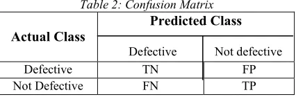
Performance is calculated accordingly to the confusion matrix shown in Table-2, which is utilized by several researchers e.g. [14], [5]. This illustrates the confusion matrix for the problem of two classes with "positive" and "negative" values class. Classifiers accuracy is measured by, "true positive rate", "false positive rate", "precision", "recall" and "F-measures" using a machine learning tool known as WEKA. This tool is a provides the groups of "machine learning algorithms" for various data mining tasks.
Table 2: Confusion Matrix
Actual Class
Predicted Class
Defective Not defective
Defective TN FP
Not Defective FN TP
Defect efficiency of software predicted based on the measure of "accuracy", "sensitivity" and "specificity" is defined as,
• Accuracy =(TP+TN) / (TP+FP+TN+FN), "The percentage of prediction that is correct".
• Sensitivity = (TP) / (TP+FN), "The percentage of positivelylabeled instances that predicted as positive".
[image:7.612.312.525.459.529.2]C. Result Evaluation
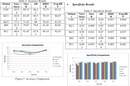
According to the best values of accuracy, we prefer 4 existing classification algorithms for comparison evaluation. All estimated values are accumulated and compared with dissimilar parameter measurement performance. The accuracy of Table-3 shows others algorithm gives a different accuracy in a different dataset. But the average performance is almost the same. The proposed RBR giving better Accuracy value in compare to existing classifier. The sensitivity and specificity measure the compute the positive and negative instances which are predicted from positive label instances as shown in Table-4 and 5. In comparison with the existing classifiers, the proposed RBP shows an average of 20% improvisation in sensitivity and 10% in case of specificity. The graphical comparison of results is presented in Figure.5, 6 and 7 in respectively.
[image:8.612.307.531.118.352.2]• Accuracy Results
Table 3: Accuracy Results Method
s
Naive bayes
Oner R
J48 RIDO
R
Prop.RB P CM1 83.9
4
89.13 86.2 3
75.73 85.32
KC1 83.0 5
83.29 85.5 6
70.15 86.87
KC2 77.5 71.25 80 76.25 81.25 JM1 81.2
8
79.67 79.8 81.42 82.02
PC1 88.8 2
91.45 87.8 3
89.14 92.43
Figure.5: Accuracy Comparison
• Sensitivity Results
Table 4: Sensitivity
Methods Naive
bayes
OnerR J48 RIDOR Prop.RBP
CM1 0.4 0.133 0.2 0.267 0.333 KC1 0.328 0.32 0.197 0.254 0.434 KC2 0.412 0.118 0.353 0.373 0.422 JM1 0.157 0.131 0.123 0.109 0.198 PC1 0.28 0.24 0.16 0.24 0.36
Figure-6.Sensitivity Comparison
• Specificity Results
Table 5: Specificity Result Method
s
Naive bayes
Oner R
J48 RIDO
R
Prop.RB P CM1 0.89
3
0.789 0.94 3
0.951 0.984
KC1 0.93 2
0.898 0.95 9
0.947 0.976
KC2 0.95 2
0.921 0.87 3
0.937 0.937
JM1 0.95 7
0.954 0.99 4
0.968 0.988
PC1 0.94 3
0.935 0.98 9
0.993 0.982
Figure-7.Specificity Comparison
5. CONCLUSION
[image:8.612.84.528.361.655.2]increase the effectiveness and quality of software development, it can take the advantage of data mining to analyze and provide a lot of data collected from defects in software development. This paper presents a rule-based prediction (RBP) method for rules that are easy to understand and have two types of exceptions that can automatically find the discovery rules, preventing the designer from doing this manually. A rule is defined as a combination of metrics/thresholds that better fits an instance of a known design defect. This proposed algorithm performs the same operation on everyone node of the "Ripple Down rule tree", which adds supplementary rules for better performance. Nevertheless, while the algorithm can fully analyze the statistics of all relevant cases, it does this in response to one bad case. This task can fully describe the effect quickly enough to change the ripple-down rule structure arbitrarily and maintain interaction development. In the experimental analysis, it shows better performance in fault prediction compared with the existing classification approach.
REFERENCES
[1] Moeyersoms J, Fortuny EJ, Dejaeger K, Baesens B, "Comprehensible software fault and effort prediction: A data mining approach" The Journal of Systems and Software. 100:80-90, Feb-2015.
[2] Y. Chen, X. Shen, Peng Du, and Bing Ge., "Research on software defect prediction based on data mining", IEEE 2nd International Conference on Computer and Automation Engineering(ICCAE),Volume 1, pages 563-567, 2010.
[3] G. Czibula, Z. Marian, I. GergelyCzibula, "Software defect prediction using relational association rule mining ", Elsevier International Journal of Information Sciences, Volume 264, April, Pages 260-278, 2014.
[4] R. Moser, W. Pedrycz, and G. Succi, "A comparative analysis of the efficiency of change metrics and static code attributes for defect prediction",ACM/IEEE 30th International Conference on Software Engineering,ICSE'08, pages 181-190, 2008.
[5] H. Zhang, X. Zhang, and Ming Gu, "Predicting defective software components from code complexity measures", IEEE In Dependable Computing Pacific Rim International Symposium on, pages 93-96, 2007.
[6] S. Lessmann, B. Baesens, C. Mues, and S. Pietsch, "Benchmarking classification models for software defect prediction: A proposed framework and novel findings",IEEE Transactions on Software Engineering, 34(4):485-496, 2008.
[7] R Geoff Dromey, "Software Control Quality - Prevention Verses Cure?", ACM Journal of Software Quality Journal archive, Volume-11 Issue 3, Pages 197-210, July 2003.
[8] Kaur S, Kumar D, "Software fault prediction in object-oriented software systems using density based clustering approach", International Journal of Research in Engineering and Technology (IJRET), 1(2):111-7, Mar-2012.
[9] Q. Song, Z. Jia, M. Shepperd, Shi Ying, and Jin Liu, "A general software defect-proneness prediction framework", Software Engineering, IEEE Transactions on, 37(3):356-370, 2011.
[10]Haghighi, A. A. S., Dezfuli, M. A., and Fakhrahmad, S. M., "Applying mining schemes to software fault prediction: A proposed approach aimed at test cost reduction", In Proceedings of the World Congress on Engineering, pp.415-419, 2012.
[11]Software Defect Dataset, PROMISE REPOSITORY, http://promise.site.uottawa.ca/ SERepository/ datasetspage.html, December 4, 2013.
[12]H. Najadat and I. Alsmadi,"Enhance Rule-Based Detection for Software Fault-Prone Modules", International Journal of Software Engineering and Its Applications,Vol. 6, No. 1, January 2012
[13]T. Hall, S. Beecham, D. Bowes, D. Gray, and S. Counsell, "A systematic literature review on fault prediction performance in software engineering", IEEE Trans. Softw. Eng., 38(6):1276– 1304, Nov. 2012.
[14]Shepperd, M., Song, Q., Sun, Z., and Mair, C., "Data Quality: Some Comments on the NASA Software Defect Data Sets", IEEE Transactions on Software Engineering, pp.1208-1215, 2013.
[15]Okutan O. T. Yildiz, "Software defect
prediction using Bayesian
networks",Inproceeding to Empirical Software Engineering, pp. 1-28, 2012.
optimization and support vector machine", IEEE 25th Chinese Control and Decision Conference (CCDC), 2013.
[17]J. Wang, B. Shen and Y. Chen, "Compressed C4.5 Models for Software Defect Prediction",IEEE 12th International Conference on Quality Software (QSIC), pp. 13-16, August2012.
[18]Z. Yan, X. Chen and P. Guo, "Software Defect Prediction Using Fuzzy Support Vector Regression", Springer-Verlag Berlin Heidelberg, 2010.
[19]E. Arisholm, L. C. Briand, and E. B. Johannessen. A systematic and comprehensive investigation of methods to build and evaluate fault prediction models. J. Syst. Softw., 83(1):2–17, Jan. 2010.
[20]Gaines, B.R., Compton, P.: Induction of Ripple-Down Rules Applied to Modeling Large Databases. J. Intell. Inf. Syst. 5(3), 211-228 ,1995.
[21]T. GalinacGrbac, P. Runeson, and D. Huljenic, "A second replicated quantitative analysis of fault distributions in complex software systems", IEEE Trans. Softw. Eng., 39(4):462– 476, Apr. 2013.
[22]D. Rodriguez, I. Herraiz, and R. Harrison, "On software engineering repositories and their open problems", In Proceedings of RAISE ’12, pages 52–56, 2012.
[23]S. Kim, T. Zimmermann, E. J. Whitehead Jr., and A. Zeller, "Predicting faults from cached history", In Proceedings of the 29th international conference on Software Engineering, ICSE '07, pages 489-498, 2007.
[24]B. Turhan, T. Menzies, A. B. Bener, and J. Di Stefano, "On the relative value of cross-company and within-cross-company data for defect prediction", Empirical Softw. Eng., 14:540-578, October 2009.
[25]Y. Ma, G. Luo, X. Zeng, and A. Chen, "Transfer learning for cross-company software defect prediction", Information Software Technology, 54(3):248–256, Mar. 2012.
[26]N. Ohlsson and H. Alberg, "Predicting fault-prone software modules in telephone switches" IEEE Trans. Softw., 22(12):886 –894, Dec. 1996.