BIROn - Birkbeck Institutional Research Online
Aksoy, Yunus and Piskorski, T. (2006) U.S. domestic money, inflation and
output. Journal of Monetary Economics 53 (2), pp. 183-197. ISSN
0304-3932.
Downloaded from:
Usage Guidelines:
Please refer to usage guidelines at or alternatively
Birkbeck ePrints: an open access repository of the
research output of Birkbeck College
http://eprints.bbk.ac.uk
Aksoy, Yunus and Piskorski, Tomasz (2006). U.S.
domestic money, inflation and output.
Journal of Monetary
Economics
53 (2), 183-197.
This is an author-produced version of a paper published in Journal of Monetary Economics (ISSN 0304-3932). This version has been
peer-reviewed but does not include the final publisher proof corrections, published layout or pagination.
All articles available through Birkbeck ePrints are protected by intellectual property law, including copyright law. Any use made of the contents should comply with the relevant law.
Citation for this version:
Aksoy, Yunus and Piskorski, Tomasz (2006). U.S. domestic money, inflation and output. London: Birkbeck ePrints. Available at:
http://eprints.bbk.ac.uk/archive/00000364
Citation for the publisher’s version:
Aksoy, Yunus and Piskorski, Tomasz (2006). U.S. domestic money, inflation and output. Journal of Monetary Economics 53 (2), 183-197.
http://eprints.bbk.ac.uk
U.S. Domestic Money, Inflation and Output
Yunus Aksoy* and Tomasz Piskorski+
Abstract
Recent empirical research documents that the strong short-term relationship between U.S. monetary aggregates on one side and inflation and real output on the other has mostly disappeared since the early 1980s. Using the direct estimate of flows of USD abroad we find that domestic money (currency corrected for the foreign holdings of dollars) contains valuable information about future movements of U.S. inflation and real output. Statistical evidence suggests that the Friedman-Schwartz stylized facts can be reestablished once the focus of analysis is back on the correct measure of domestic monetary aggregates.
JEL Classification: E3, E4, E5.
Keywords: foreign holdings, domestic money, monetary aggregates, information value.
*Yunus Aksoy: Birkbeck College, University of London, Malet Street, London, WC1E 7HX United Kingdom, Phone: (020) 7631 6407, Fax: (020) 7631 6416.
+ Tomasz Piskorski: Department of Economics, Stern School of Business, New York University, 44 West 4th Street, New York, NY 10012, USA, e-mail: tp431@nyu.edu;
We are grateful to Richard Porter, Richard Anderson and Philip Jefferson for providing the foreign holdings data. We are particularly grateful to the editor Robert King, an anonymous referee of the journal, Richard Anderson, Elena Bisagni, Fabio Canova, Alan Carruth, Günter Coenen, Ben Craig, Paul De Grauwe, Hans Dewachter, Ruth Judson, Siem Jan Koopman, Hanno Lustig, Helmut Lütkepohl, Dieter Nautz, Athanasios Orphanides, Richard Porter, Volker Wieland and to participants at the seminars held at the European Central Bank, universities of
Leuven, Sabancı, Koç, Boğaziçi, Amsterdam, Frankfurt and Kent, the ESEM and EEA 2001 meetings in Lausanne
1. Introduction
One of the long-standing empirical problems in macroeconomics has been whether money
has a significant and stable relationship with aggregate output and inflation. Recent empirical
research finds that, since the early 1980s the strong positive short-term relationship between U.S.
monetary aggregates and real output as outlined in the classic study by M. Friedman and Schwartz
(1963) has mostly disappeared. In contrast, short-term interest rates are found containing valuable
lead information for real output. Remarkably, this research documents that monetary aggregates as
well as short-term interest rates are very poor indicators for U.S. inflation over the last two
decades.1
In this paper, we argue that the international currency feature of the U.S. dollar generates
substantial noise when monetary aggregates are used to assess domestic macroeconomic conditions.
The crucial question that arises here is the extent to which correcting the U.S. monetary aggregates
for the foreign holdings component affects the time series properties of monetary aggregates.
Jefferson (2000) provides a quantitative assessment of the importance of accounting for foreign
holdings of U.S. currency for the U.S. nominal income in the context of McCallum monetary base
rule for the period 1981:1-1995:4. 2 He finds that the foreign holdings corrected monetary base has
more explanatory power for changes in nominal income than when the total base is used.
We focus on two other key macroeconomic fundamentals: real output and inflation. Using
recent quarterly data for flows of U.S. dollars abroad for the period 1965:1-1998:2, we find that the
apparent lack of a significant relationship between U.S. monetary aggregates on one side and real
output and inflation on the other is partially attributable to the presence of substantial and unstable
foreign holdings of the U.S. dollar, which are largely unaccounted for.
1 See for example Bernanke and Blinder (1992), Friedman and Kuttner (1992, 1996), Estrella and Mishkin (1997),
Friedman (1998), Stock and Watson (2001).
2 First quarter of 1981 to fourth quarter of 1995.
The paper is organized as follows. Section 2 provides the intuition behind the relevance of
correcting U.S. monetary aggregates for the foreign holdings of dollars and presents the data.
Section 3 presents the entire dataset used in the paper. Section 4 compares the performance of the
corrected monetary aggregate, domestic money, with uncorrected monetary aggregates and the
Federal Funds rate to predict U.S. inflation and real output growth in Granger-style regressions.
Section 5 presents stability tests. Section 6 presents the Granger causality tests based on inflation
and real output equations that include domestic money and other monetary aggregates together with
the Federal Funds rate. Finally, Section 7 concludes.
2. Foreign Holdings of U.S. Dollars
The U.S. dollar is the most important international currency. Private individuals, central
banks, commercial banks and firms in foreign countries use significant amounts of U.S. dollars. U.S.
dollars are used for international trade purposes and central bank interventions. Furthermore, in
most developing countries the dollar is seen as an investment opportunity to immunize citizens'
wealth from domestic nominal and real shocks. It is even used in daily transactions.
If there were no competing international currencies that could substitute these holdings and
no abrupt shifts in the currency preferences of foreigners so that domestic stabilization objectives
would not be endangered, than any rational central bank would like to satisfy the currency demands
outside its borders to generate seignorage output.3
Monetary policymakers and market analysts want to know the amount and flow dynamics of
currency abroad in order to be able to assess its implications for the state of the domestic monetary
and real economic environment. If the currency flows abroad are large, unstable and unaccounted
3 Based on the estimates of foreign holdings by Porter and Judson (1996), Obstfeld and Rogoff (1996) and Jefferson
(1998) calculated the amount of seigniorage revenues obtained by the U.S. Federal Reserve to be between 20 and 30 billion dollars per year.
for, then the interpretation of domestic monetary conditions might be severely complicated and even
turn out to be spurious.
The crucial question concerns the measurement of foreign holdings. Several studies have
focused recently on this issue.4 In this paper we will use the shipment proxy method, which is
published officially by the Board of Governors of the Federal Reserve System in its Flow of Funds
accounts and by the Department of Commerce’s Bureau of Economic Analysis (BEA) in its
International Investment Position of the United States. The published series represents an estimate
of wholesale currency shipments abroad. This consists of net shipments of $100s from the New
York City and Los Angeles cash offices of the Federal Reserve district banks. The assumption
underlying this method is that mostly lower denomination notes ($5s, $10s, $20s and $50s) circulate
in the U.S. economy, whereas mostly $100 notes circulate abroad.5 It is important to stress that the
shipment proxy is a direct method, therefore the process of collecting data on the flows of U.S.
dollars abroad is a matter of accountancy and clearly exogenous to U.S. economic conditions.
[Insert Figure 1]
On the left hand-side of Figure 1 we present the flow estimate of U.S. dollars abroad at an
annual frequency. On the right hand-side, we present the ratio of changes in the foreign holdings
abroad to the total change in the currency on an annual basis (calculated as 100 × [flows
abroad/change in currency]). As we observe, the flows of U.S. dollars abroad were increasing in an
4 See Feige (1996), Porter and Judson (1996), Doyle (2000) and Anderson and Rasche (2000).
5 Bach (1997) reports that several of the institutional characteristics of the circulation of U.S. currency support shipment
proxy. He indicates that mostly lower denomination notes ($5s, $10s, $20s, and $50s) circulate in the U.S. economy, whereas mostly $100 notes circulate abroad. As an example he cites a 1995 survey of U.S. households, which found that U.S. households could account at most for a little more than 3 percent of total holdings of $100 notes. Second, Porter and Judson (2001) report that about 90 percent of wholesale shipments are $100s and the vast majority of these appear to originate and return to the New York City Federal Reserve Cash Office. Bach (1997) reports that the inclusion of the Los Angeles Cash Office is based on information that suggests that $100 notes returned to the United States from abroad (largely from Asian countries) are shipped primarily to Los Angeles. That is why only shipments from the New York and Los Angeles Cash Offices are relevant. Finally, Porter and Judson (1996) found that wholesale currency shipments that move through the international banking constitute the vast majority of all international currency
unstable way over the period 1965-1998. The flows of U.S. currency abroad are much higher in the
1990s as compared to the previous decades.6
However, what really matters is the ratio of foreign flows to changes of the currency. If this
ratio were constant over time, the correction for foreign flows would not affect the time series
properties of money growth rate. In other words, in this case the percentage change in the total
money in circulation would be equal to the percentage change in currency that remains within U.S.
borders.7 On the other hand, if the ratio of foreign flows to changes of currency is large and
unstable, the use of uncorrected money growth rates in assessing domestic economic conditions will
very likely lead to spurious evidence. As we observe, the right hand figure indicates that the ratio of
foreign flows to the total change in the currency is large, unstable, and steadily increasing.
To assess empirically the importance of foreign holdings of U.S. dollars, a "corrected"
monetary aggregate must be constructed. We opt to correct only currency for foreign holdings in
order to obtain a realistic measure of the U.S. domestic narrow money supply. It is a simple
monetary aggregate not based on estimation so that its amount is determined and precisely known
by the monetary authority.8
shipments, with relatively minor amounts being carried by individuals, firms, and smaller financial institutions. See also Feige (1996) and Anderson and Rasche (2000) for more discussion.
6 Porter and Judson (1996) explain the very strong increase in the foreign holdings of the U.S. dollar in the 1990s by the
Westward opening of the Eastern European countries and Russia, and instability in the Latin American economies. Recent estimates show that in Russia the level of U.S. dollar holdings is about 60 billion dollars (See U.S. Treasury, 2000). These holdings mainly reflect efforts by residents of some countries with high financial instability to substitute a more stable dollar for their own currency and therefore are not necessarily linked to U.S. domestic conditions.
7 In this case, the share of currency in circulation abroad of the total currency in circulation would also be constant and
equal to the ratio of foreign flows to the change of the total currency.
8 In principle, all monetary aggregates can be corrected for the foreign holdings noise. However, all money measures
beyond the narrow definitions of monetary aggregates contain dynamics arising from the financial sector and are typically compounded by market forces. A correction of such aggregates is extremely difficult. Secondly, other potential candidates such as the monetary base measures are estimates and not accounting figures. This results in considerable differences between two well-known measures, the Board of Governors' monetary base and the Federal Reserve of St. Louis monetary base.
The data for flows of U.S. dollars abroad covers the sample period 1965:1-1998:2. We do
not consider the most recent available data for foreign flows. As reported by Judson and Porter
(2001) and Lambert and Stanton (2001) the domestic currency demand temporarily surged in
preparation for the century date change, which could introduce a large anomaly in the foreign flows
estimate.
We calculate domestic money (Mdt- foreign holdings corrected currency) as follows:
t t t C FH
Md = − (1)
where is the level of currency at time t (measured quarterly in billions of dollars) and is the
level of dollar holdings outside the United States at time t (measured quarterly in billions of dollars).
t
C FHt
In order to subtract accumulated flows of U.S. dollars abroad from the total level of
currency, the amount of foreign holdings of U.S. dollars in 1964:4 must be known. However, there
is no official data on the amount of foreign holdings in 1964:4. As the stock estimate of domestic
money given by (1) is conditional on the selected initial benchmark, throughout this paper we will
always report statistical evidence for alternative assumptions on the initial level of U.S. dollar stock
abroad. For this purpose, we assume five different initial foreign holdings levels in 1964:4 (ranging
from 0% to 40% of the total currency, at 10% intervals). This will enable us to assess the robustness
of our results with respect to various assumed levels of foreign holdings in 1964:4. 9
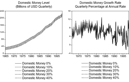
[Insert Figure 2]
The left-hand side of Figure 2 shows the level of domestic money and the right-hand side
displays quarterly growth of domestic currency for different initial level assumptions for foreign
holdings. As of the beginning of the 1980s, the small discrepancy in growth rates due to initial level
assumptions diminishes. We obtain nearly a single series for the domestic money growth rate.
9 As noted in a separate appendix to Anderson and Rasche (2000), the assumption of 40% of the total currency being
held abroad in the 1960s is highly implausible. As an example, in 1960 40% of the total currency equals the sum of all $100 and $50 notes plus about one-half of the $20 notes in circulation at that time (see Banking and Monetary Statistics 1941-1970). Therefore, the assumption of 40% of the total currency being held abroad in 1964:4 may be treated as a maximum threshold for foreign holdings in 1964:4 while the 0% assumption constitutes the natural minimum level.
3. Data
The quarterly data covers the period 1965:1-1998:2.10 We will study the following
macroeconomic fundamentals (in natural log differences): real output represented by real GNP and
inflation represented by the GNP deflator.11 The financial variables to assess the fluctuations of the
macroeconomic variables that we consider consist of the monetary aggregates (in natural log
differences) and the Federal Funds rate (in the first difference form) and are as follows: “corrected”
domestic money (Δln(Md)), currency (Δln(C)), monetary base measures of the Board of Governors
of the Federal Reserve System (Δln(BGbase)) and of the Federal Reserve Bank of St. Louis
(Δln(SLbase)), M1 (Δln(M1)), M2 (Δln(M2)), the Federal Funds rate (ΔFUNDS). All series satisfy
stationarity properties.12
4. Granger Causality Tests
The autoregressive specification for real output changes and inflation follows exactly
Friedman and Kuttner (1992). The specification for real output changes (Δy) is given by:
t i i t i i i t i i i t i
t y p m v
y = + Δ + Δ + Δ +
Δ
∑
∑
∑
= − = − = − 4 1 4 1 4 1 δ λ β α (2)
where Δy, Δp, and Δm are the growth rates of real output (one-quarter log differences of real GNP in
annual terms), inflation (one-quarter log differences of GNP deflator in annual terms), and the
10 Detailed data descriptions and source references are tabulated in the Appendix.
11 In the sample period under investigation, the correlation between the quarterly growth rates of chained 1996 dollars
seasonally adjusted GDP and GNP at annual rate is 0.994; and the correlation between the GDP deflator and the GNP deflator is 0.999. Therefore, the results reported in the paper are robust with respect to the choice of the real output measure.
12 Both Dickey-Fuller and Phillips-Perron tests reject the null hypothesis of unit root for all the mentioned series'
specifications.
change in the alternative financial variables we will use (the one-quarter growth rate of a monetary
aggregate or the one-quarter difference in the Federal Funds rate, measured in annually),
respectively.
The three-variable specification for inflation takes the following form:
t i i t i i i t i i i t i
t p y m v
p = + Δ + Δ + Δ +
Δ
∑
∑
∑
= − = − = − 4 1 4 1 4 1 δ λ β α (3)
where now, Δp, Δy, and Δm are inflation (the one-quarter log difference of GNP deflator in annual
terms), the growth rate of real output (the one-quarter log difference of real GNP in annual terms),
and the change in the financial variable we will use (the one-quarter growth rate of the monetary
aggregate or the one-quarter difference of the Federal Funds rate, measured annually), respectively.
[Insert Table 1]
Table 1 presents the p-values of the Granger causality χ-square statistics13 computed with
White (1980) heteroskedasticity consistent standard errors.14 The null hypothesis is that all
coefficients on the lagged financial variables, considered individually in the autoregressive
specifications, are zero. The table presents results for the period 1966:2-1998:2 and for the period
1980:1-1998:2. The latter period corresponds to the last two decades during which the relationship
between monetary aggregates and macroeconomic fundamentals were documented to fail.
Real Output: Over the entire sample period 1966:2-1998:2, domestic money is significant at
1% for 0%, 10% and 20% initial level assumption (5% for 30% and 40% initial level assumption).
The Board of Governors monetary base is significant at 5% and M2 is significant at 1%, whereas the
13 The Granger causality test statistics based on the F-statistics yield very similar p-values to those based on the χ-square
statistics.
14 The White test for heteroskedasticity rejected the non-constancy of the residual variance for almost all-financial
variables in the specifications (2) and (3). Therefore, throughout the paper the White heteroskedasticity-consistent standard errors are used to derive the corresponding χ-square statistics of the Granger causality tests. Moreover, the relative performance of alternative financial variables in terms of the heteroskedasticity consistent Granger causality statistics is very similar to those based on the statistics computed with unadjusted OLS residuals. Finally, we note that the Ljung-Box Q-statistics do not reject the null hypothesis that there is no autocorrelation in the residuals of the equations (2) to (3) for all financial variables considered.
other standard monetary aggregates exhibit no significant predictive content. In addition, the Federal
Funds rate has high significance in the real output equation.
In the period 1980:1-1998:2, in contrast to the poor performance of narrow monetary
aggregates, domestic money contains significant predictive content for the real output (at 1%). We
find that M2 is also significant, although now at 5%. Other standard monetary aggregates, including
the Board of Governors monetary base, exhibit no significant predictive content for the output
movements in the sample period 1980:1-1998:2. Table 1 confirms Friedman and Kuttner’s (1992)
and Estrella and Mishkin’s (1997) indication of the collapse of the information content of the
uncorrected monetary aggregates after the 1980’s. Note that the Federal Funds rate is significant at
1%.
Inflation: For the period 1966:2-1998:2 domestic money contains significant information for
future fluctuations in inflation (at 5%). Among the standard monetary aggregates, only the Board of
Governors monetary base is significant (at 10%). The Federal Funds rate contains significant
information at 10%.
In the period 1980:1-1998:2, in contrast to the very poor performance of all the standard
financial variables over the period of the last two decades, domestic money is significant in the
inflation equation (at 1%).15
We also note that the sum of coefficients on domestic money is positive in the real output as
well as in the inflation equation in both sample periods.
15 Note also that variance decompositions of inflation and real output based on unconstrained VAR representations
indicate that domestic money accounts for a substantial part of the forecast error variance of inflation and real output. For the sake of brevity, we do not report the results here but they are available from the authors.
5. Stability Tests
To analyze the stability of the output and inflation relationships we conduct several exercises
based on: recursive p-values, formal coefficient stability tests and an out-of-sample forecasting
exercise.
Recursive p-values. First, we graphically explore the stability of p-values. For this purpose
we present a series of p-values of Granger causality statistics for the coefficients of the alternative
financial variables obtained from recursive estimations for real output and inflation. Two recursive
estimations are considered. In the first exercise, the endpoint of the entire sample period (1998:2) is
held fixed, while in the second one the beginning of the entire sample period (1966:2) remains
unchanged.
Figures 3a and 4a display recursive p-values for the Granger causality tests for real output
and inflation over the sample periods ending in 1998:2 for alternative financial variables and
domestic money with different assumptions on the initial level. The first p-value plotted in each
graph of the figures gives the Granger causality test statistics for the sample period 1966:2-1998:2,
and the subsequent p-values refer to the reduced samples 1966:3-1998:2, 1966:4-1998:2, and so on
with the last value corresponding to the sample period 1988:2-1998:2.
Figures 3b and 4b present the recursive p-values of the coefficients of the financial variables
for Granger causality tests of real output and inflation, respectively, over the sample periods starting
at 1966:2. The first p-value plotted in the figures displays the Granger causality test statistics for the
sample period 1976:2, and the subsequent p-values refer to the expanded samples
1966:2-1976:3, 1966:2-1976:4, and so on, with the last value corresponding to the entire sample period
1966:2-1998:2. The two dashed lines correspond to the 5% and 10% significance level.16
[Insert Figures 3a and 3b]
Figures 3a and 3b represent the p-values for real output. Figure 3a shows that domestic
16 In the recursive regressions, the minimum sample period equals 10 years.
money is significant in the real output equation for the entire series of estimations with starting point
ranging from 1966:2 to 1988:2 and the sample endpoint 1998:2 held fixed. This result holds for
alternative initial level assumptions. All the other narrow monetary aggregates perform very poorly
when compared to domestic money. Even the Federal Funds rate performs badly when earlier
periods up to 1983 are excluded from the estimations.
Figure 3b shows that domestic money contains significant information on U.S. real output
when estimations capture quarters beyond 1982:1. In other words, we find that when the 1960s and
1970s are always included in the sample a significant relationship between real output and domestic
money is established after the inclusion of the observations as of 1982. These results hold
irrespective of the initial level assumption. Among the standard monetary aggregates, M2 contains
valuable information over the entire sequence of estimations, whereas the Board of Governors
monetary base displays significant information when observations as of 1982:1 are included. Other
measures of monetary aggregates perform very poorly, violating the Friedman-Schwartz results. We
also observe that the Federal Funds rate is significant in the real output equation for all estimations
when the sample size is extended (having 1966:2 fixed).
[Insert Figures 4a and 4b]
Figures 4a and 4b display the corresponding p-values of the coefficients of financial
variables for U.S. inflation. Figure 4a shows clear evidence of significant information content of
domestic money for almost all recursive estimations conducted (where the 1998:2 sample endpoint
is fixed). This result holds irrespective of the assumption on the initial level of foreign holdings. In
contrast, all standard financial variables considered, including the Federal Funds rate, display
insignificant relationships with U.S. inflation in most of the estimations.
Figure 4b indicates that when we fix the beginning of the sample to equal 1966:2 and add
observations consecutively, domestic money only contains significant information when the sample
captures observations from the late 1990s onwards. We note that the standard uncorrected monetary
aggregates perform poorly in explaining inflation with the exception of the Board of Governors
adjusted monetary base. We also note that the Federal Funds rate contains significant information in
most of the periods after 1982.
Formal Stability Tests: Next, in order to formally assess the stability of the coefficients of
the Granger causality specifications we perform the full sample stability tests. Three types of tests
are considered: the Quandt likelihood ratio (QLR) statistic in Wald form, the mean Wald statistic
(Hansen (1992), Andrews and Ploberger (1994)), and the Andrews and Ploberger (1994)
exponential average Wald statistic. We derive these statistics from the recursive Wald tests with
White (1980) heteroskedasticity standard errors for changes in the constant term and four
autoregressive coefficients of the financial variable. We use 30% symmetric trimming to allow
testing for a breakpoint in the interval, 1976:1-1988:4. The results of the stability tests are displayed
in Table 2.
[Insert Table 2]
There is no evidence against the stability of the relationship between real output and
domestic money. In contrast, there is evidence against the null of parameter stability in the real
output equation for most of the standard financial variables. Only in the case of M2 and the St.
Louis adjusted monetary base is the null of no single breakpoint not rejected. Domestic money also
displays one of the smallest Wald statistics among all financial variables considered together with
the monetary base of the Federal Reserve Bank of St. Louis.
In the case of inflation, the hypothesis of coefficient stability for domestic money is not
rejected for various initial level assumptions (the only exception being domestic money with 0%
initial level assumption where sup-Wald and exp-Wald indicate the rejection of stability at 5%).
The tests reject the null of stability for the coefficients of both monetary base measures and
currency.
Out-of-sample forecasting. In Table 3, we present the root mean squared errors (RMSE)
results for the one step ahead out of sample predictions. We split the entire sample period in two
equal parts of sixteen years (64 versus 65 observations). Therefore, the first initial estimation is
performed for the 1966:2-1982:1 period. Then we expand our sample by adding recursively
subsequent observations. We make one quarter ahead predictions for real output and inflation. The
predictions are made for the quarters ranging from 1982:2 until 1998:2.
[Insert Table 3]
For the case of real output Table 3 shows that domestic money displays the smallest RMSE
among the monetary aggregates. In the case of inflation, domestic money shows the smallest RMSE
among all financial variables considered. The strong performance of domestic money is not affected
by the alternative assumptions concerning the level of foreign holdings in 1964:4.
6. Performance of Monetary Aggregates in the Presence of the Federal Funds rate
As a final step, we assess whether the monetary aggregates contain any significant
information value conditional on the presence of the Federal Funds rate. We re-estimate
specifications (2) and (3), now including a monetary aggregate together with the Federal Funds rate
(with four lags). The results are shown in Table 4.
[Insert Table 4]
Real Output: For the entire sample period, 1966:2-1998:2, only the monetary base measure
of the Board of Governors is significant in the real output equation (at 5%) given the presence of the
Federal Funds rate. In the second sub-sample (1980:1-1998:2), domestic money is significant in the
presence of the Federal Funds rate (at 1%) as well as the Board of Governor’s monetary base (at
5%). Other standard monetary aggregates display no significance.
Inflation: For the entire sample, only domestic money and the Board of Governor’s monetary
base contain statistically significant information additional to the Federal Funds rate (at 5% and at
10% respectively). In the second sample (1980:1-1998:2), domestic money is significant at 1% and
the Board of Governor’s monetary base is significant at 10%. Alternative assumptions on the initial
level of foreign holdings do not affect any of these results.
We also note that the sum of coefficients on domestic money is positive in the real output as
well as the inflation equation including the Federal Funds rate in both sample periods.
7. Concluding Remarks
We find that currency corrected for foreign holdings has increased marginal predictive
content for U.S. inflation and output relative to standard unadjusted money series. These findings
can be interpreted as providing support to the Friedman-Schwartz stylized facts on the close
relationship between monetary aggregates and macroeconomic fundamentals. A practical use of the
corrected monetary aggregate in actual monetary policymaking would strongly rely on the accuracy
and the timeliness of the measurement of the flows of currency abroad.
References:
Anderson, R.G. and R.H. Rasche, 2000, The domestic adjusted monetary base, Federal Bank of St.
Louis Working Paper, 2000-002.
Andrews, D.W.K., 1993, Tests for parameter instability and structural change with unknown change
point, Econometrica 61, 821-856.
Andrews, D.W.K. and W. Ploberger, 1994, Optimal tests when a nuisance parameter is present only
under the alternative, Econometrica 62, 1383-1414.
Bach, C.L., 1997, U.S. international transactions, revised estimates for 1974-96, Survey of Current
Business 77, 43-55.
Bernanke, B.S. and A.S. Blinder, 1992, The Federal Funds rate and the channels of monetary
transmissions, American Economic Review 82, 901-921.
Board of Governors of the Federal Reserve System, (1976), Banking and Monetary Statistics
1941-1970, Board of Governors of the Federal Reserve System, Washington, 1168 p.
Doyle, B.M., 2000, ‘Here dollars, dollars…’- estimating currency demand and worldwide currency
substitution, Board of Governors of the Federal Reserve System, International Finance Discussion
Paper 657.
Estrella, A. and F.S. Mishkin, 1997, Is there a role for monetary aggregates in the conduct of
monetary policy?, Journal of Monetary Economics 40, 279-304.
Feige, E.L., 1996, Overseas holdings of U.S. currency and the underground economy, in: S. Pozo,
ed., Exploring the underground economy (W.E. Upjohn Institute for Employment Research,
Kalamazoo, Michigan) 5-62.
Friedman, B.M., 1998, The rise and fall of money growth targets as guidelines for U.S. monetary
policy, NBER Working Paper 5465.
Friedman, B.M. and K.N. Kuttner, 1992, Money, income, prices and interest rates, American
Economic Review 82, 472-492.
Friedman, B.M. and K.N. Kuttner, 1996, A price target for U.S. monetary policy? Lessons from the
experience with money growth targets, Brookings Papers on Economic Activity, 77-146.
Friedman, M. and A.J. Schwartz, 1963, A monetary history of the United States: 1867-1960
(Princeton University Press, Princeton New Jersey).
Hansen, B.E., 1992, Tests for parameter instability in regressions with I(1) processes, Journal of
Business and Economic Statistics 10, 321-336.
Jefferson, P.N., 1998, Seignorage payments for the use of the dollar: 1977-1995, Economics Letters
58, 225-230.
Jefferson, P.N., 2000, Home base and monetary base rules: Elementary evidence from the 1980s and
1990s, Journal of Economics and Business 52, 161-180.
Judson, R.A. and R.D. Porter, 2001, Overseas dollar holdings: What do we know?,
Wirtschaftspolitische Blatter 48, 431-440.
Lambert, M.J. and D. Stanton, 2001, Opportunities and challenges of the U.S. dollar as an
increasingly global currency: A Federal Reserve perspective, Federal Reserve Bulletin 87, 567-575.
Obstfeld, M. and K. Rogoff, 1996, Foundations of international macroeconomics (MIT Press,
Cambridge, Massachusetts).
Porter, R.D. and R.A. Judson, 1996, The location of U.S. currency: How much is abroad?, Federal
Reserve Bulletin 82, 883-903.
Stock, J.H. and M.W. Watson, 2001, Forecasting output and inflation: The role of asset prices,
NBER Working Paper 8180.
United States Treasury Department, 2000, The use and counterfeiting of United States currency
abroad, http://www.federalreserve.gov/boarddocs/RptCongress/counterfeit.pdf.
White, H., 1980, A heteroskedasticity-consistent covariance matrix and a direct test for
heteroskedasticity, Econometrica 48, 817-838.
Appendix
Data Sources:
Flow of Funds Accounts, Federal Reserve Board of Governors: Flow Estimate of U.S. Dollars
Abroad - Billions of Dollars.
Federal Reserve Board of Governors: Currency- M1 Currency Component, Billions of Dollars,
Seasonally Adjusted; Board of Governors' Adjusted Monetary Base- Billions of Dollars, Seasonally
Adjusted; M1 Money Stock- Billions of Dollars, Seasonally Adjusted; M2 Money Stock-Billions of
Dollars, Seasonally Adjusted; Federal Funds Rate- Percentage Points at Annual Rate.
Federal Reserve Bank of St. Louis: St. Louis Adjusted Monetary Base- Billions of Dollars,
Seasonally Adjusted.
U.S. Department of Commerce, Bureau of Economic Analysis: Real Gross National Product
-Billions of Chained 1996 Dollars Seasonally Adjusted Annual Rate; Implicit Price Deflator Gross
National Product-Seasonally Adjusted 1996=100.
Table 1: P-Values: Granger Causality χ-Square Statistics (OLS Estimates, White Heteroskedasticity Consistent Standard Errors)
Real Output Equation Inflation Equation
1966:2-1998:2 1980:1-1998:2 1966:2-1998:2 1980:1-1998:2
Variable χ-square χ-square χ-square χ-square
Domestic Money
) ln(Md
Δ 0% 0.006 0.002 0.029 0.009
) ln(Md
Δ 10% 0.006 0.001 0.026 0.009
) ln(Md
Δ 20% 0.007 0.001 0.025 0.009
) ln(Md
Δ 30% 0.011 0.001 0.025 0.009
) ln(Md
Δ 40% 0.022 0.001 0.029 0.009
Uncorrected Monetary Aggregates and Federal Funds Rate
) ln(C
Δ 0.829 0.677 0.288 0.449
) ln(BGbase
Δ 0.045 0.104 0.073 0.242
) ln(SLbase
Δ 0.768 0.295 0.380 0.448
) 1 ln(M
Δ 0.140 0.130 0.485 0.583
) 2 ln(M
Δ 0.000 0.020 0.421 0.840
FUNDS
Δ 0.000 0.000 0.053 0.168
Table 2: Tests for Structural Change (30% Symmetric Trimming)
Tests are significant at * 10 percent; ** 5 percent; *** 1 percent. Critical values for the sup-Wald statistics are tabulated in Andrews (1993). Critical values for the mean-Wald and the exponential average Wald statistics are tabulated in Andrews and Ploberger (1994).
Real Output Equation Inflation Equation
Test Statistics Test Statistics
Variable sup-Wald mean-Wald exp-Wald sup-Wald mean-Wald exp-Wald
Domestic Money )
ln(Md
Δ 0% 10.89 4.81 3.75 17.00** 6.60 6.14**
) ln(Md
Δ 10% 9.01 4.10 3.02 14.30 5.90 4.87
) ln(Md
Δ 20% 6.92 3.29 2.25 11.32 5.21 3.71
) ln(Md
Δ 30% 4.77 2.45 1.50 8.99 4.61 2.87
) ln(Md
Δ 40% 2.98 1.77 0.94 8.57 4.16 2.44
Uncorrected Monetary Aggregates and Federal Funds Rate
) ln(BGbase Δ ) ln(SLbase Δ ) 1 ln(M Δ ) 2 ln(M Δ FUNDS Δ ) ln(C
Δ 16.38* 6.76 5.95** 23.92*** 9.83** 8.58***
14.49 5.98 5.18* 27.62*** 15.90*** 11.22***
9.26 4.64 2.91 15.52* 9.31* 6.21**
16.64** 10.25** 6.43** 8.66 6.18 3.26
11.40 7.24 4.32 6.44 3.82 2.15
Table 3: Root Mean Squared Errors Predictions for: 1982:02-1998:02
Real Output Equation
) ln(Md Δ 0% ) ln(Md Δ 10% ) ln(Md Δ 20% ) ln(Md Δ 30% ) ln(Md Δ
40% Δln(C) ln( )
BGbase
Δ Δln(SLbase) Δln(M1) Δln(M2) ΔFUNDS
2.51 2.45 2.40 2.35 2.31 2.96 2.69 2.65 2.96 2.64 2.17
Inflation Equation ) ln(Md Δ 0% ) ln(Md Δ 10% ) ln(Md Δ 20% ) ln(Md Δ 30% ) ln(Md Δ
40% Δln(C) Δln(BGbase)
)
ln(SLbase
Δ Δln(M1) Δln(M2) ΔFUNDS
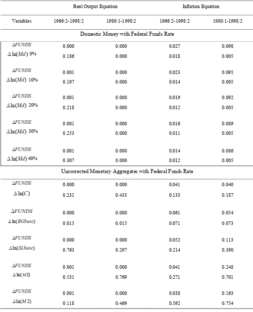
Table 4: P-Values: Granger Causality χ-Square Statistics
Equations that Include the Federal Funds Rate Together with a Monetary Aggregate (OLS Estimates, White Heteroskedasticity Consistent Standard Errors)
Real Output Equation Inflation Equation
Variables 1966:2-1998:2 1980:1-1998:2 1966:2-1998:2 1980:1-1998:2
Domestic Money with Federal Funds Rate
FUNDS
Δ 0.000 0.000 0.027 0.098
) ln(Md
Δ 0% 0.186 0.000 0.018 0.005
FUNDS
Δ 0.001 0.000 0.023 0.095
) ln(Md
Δ 10% 0.197 0.000 0.014 0.005
FUNDS
Δ 0.001 0.000 0.019 0.092
) ln(Md
Δ 20% 0.218 0.000 0.012 0.005
FUNDS
Δ 0.001 0.000 0.016 0.089
) ln(Md
Δ 30% 0.253 0.000 0.011 0.005
FUNDS
Δ 0.001 0.000 0.014 0.086
) ln(Md
Δ 40% 0.307 0.000 0.012 0.005
Uncorrected Monetary Aggregates with Federal Funds Rate
FUNDS
Δ 0.000 0.000 0.041 0.040
) ln(C
Δ 0.231 0.433 0.133 0.187
FUNDS
Δ 0.000 0.000 0.061 0.054
) ln(BGbase
Δ 0.015 0.015 0.071 0.073
FUNDS
Δ 0.000 0.000 0.052 0.113
) ln(SLbase
Δ 0.763 0.297 0.214 0.390
FUNDS
Δ 0.001 0.000 0.041 0.248
) 1 ln(M
Δ 0.531 0.769 0.271 0.701
FUNDS
Δ 0.001 0.000 0.038 0.163
) 2 ln(M
Figure 1
0 5 10 15 20 25
1965 1970 1975 1980 1985 1990 1995
Flow of U.S. Dollars Abroad (Billions of USD Annually)
0 10 20 30 40 50 60 70 80 90
1965 1970 1975 1980 1985 1990 1995
Note: Domestic money X% stands for the foreign holdings corrected currency with an initial level assumption of X% of the currency being held abroad at the 1964:4 period.
120 160 200 240
40 80
0
Figure 2
[image:25.595.73.512.90.370.2]1965 1970 1975 1980 1985 1990 1995
Domestic Money 0% Domestic Money 10% Domestic Money 20% Domestic Money 30% Domestic Money 40% Domestic Money Level (Billions of USD Quarterly)
-4 12 16
0 4 8
1970 1975 1980 1985 1990 1995