Pricing in electricity markets: a mean reverting jump diffusion model with seasonality

BIROn - Birkbeck Institutional Research Online

Cartea, Alvaro and Figueroa, M.G. (2005) Pricing in electricity markets:

a mean reverting jump diffusion model with seasonality. Working Paper.

Birkbeck, University of London, London, UK.

Downloaded from:

Usage Guidelines:

Please refer to usage guidelines at or alternatively

ISSN 1745-8587

Birkbeck Workin

g

Pa

p

ers in Economics & Finance

School of Economics, Mathematics and Statistics

BWPEF 0507

Pricing in Electricity Markets: a mean

reverting jump diffusion model with

seasonality

Álvaro Cartea

Marcelo G Figueroa

Pricing in Electricity Markets: a mean reverting

jump diffusion model with seasonality

´

Alvaro Cartea and Marcelo G. Figueroa

Birkbeck College, University of London

January 19, 2005

Abstract

In this paper we present a mean-reverting jump diffusion model for the elec-tricity spot price and derive the corresponding forward in closed-form. Based on historical spot data and forward data from England and Wales we calibrate the model and present months, quarters, and seasons–ahead forward surfaces.

Keywords: Energy derivatives, electricity, forward curve, forward surfaces.

1

Introduction

One of the key aspects towards a competitive market is deregulation. In most elec-tricity markets, this has however only occurred recently. Prior to this, price variations were often minimal and heavily controlled by regulators. In England and Wales in particular, prices were set by the Electricity Pool, where due to centralisation and inflexible arrangements prices failed to reflect falling costs and competition. Deregu-lation came by the recent introduction on March 27, 2001 of NETA (New Electricity Trade Arrangement), removing price controls and openly encouraging competition.

Price variations have increased significantly as a consequence of the introduction of competition, encouraging the pricing of a new breed of energy-based financial products

∗_{Email: a.cartea@bbk.ac.uk and m.figueroa@econ.bbk.ac.uk. First version, June 2004. We are}

to hedge the inherent risk, both physical and financial, in this market. Most of the current transactions of instruments in the electricity markets is carried out through bilateral contracts ahead of time although electricity is also traded on forward and futures markets and through power exchanges.

One of the most striking differences that singles out electricity markets is that elec-tricity is very difficult or too expensive to store, hence markets must be kept in balance on a second-by-second basis. In England and Wales, this is done by the National Grid Company which operates a balancing mechanism to ensure system security.1

More-over, although power markets may have certain similarities with other markets, they present intrinsic characteristics which distinguish them. Two distinctive features are present in energy markets in general, and are very evident in electricity markets in particular: the mean reverting nature of spot prices and the existence of jumps or spikes in the prices.

In stock markets, prices are allowed to evolve ‘freely’, but this is not true for electricity prices; these will generally gravitate around the cost of production. Under abnormal market conditions, price spreads are observed in the short run, but in the long run supply will be adjusted and prices will move towards the level dictated by the cost of production. This adjustment can be captured by mean-reverting processes, which in turn may be combined with jumps to account for the observed spikes.

Therefore, to price energy derivatives it is essential that the most important char-acteristics of the evolution of the spot, and consequently the forward, are captured. Several approaches may be taken, generally falling into two classes of models: spot-based models and forward-spot-based models. Spot models are appealing since they tend to be quite tractable and also allow for a good mathematical description of the prob-lem in question. Significant contributions have been made by Schwartz, in [16] for instance the author introduces an Ornstein-Uhlenbeck type of model which accounts for the mean reversion of prices, and in [12] Luc´ıa and Schwartz extend the range of these models to two-factor models which incorporate a deterministic seasonal com-ponent. On the other hand forward-based models have been used largely in the Nord Pool Market of the Scandinavian countries. These rely heavily, however, on a large data set, which is a limiting constraint in the case of England and Wales. Finally, it must also be pointed out that the choice of model may sometimes be driven by what kind of information is required. For example, pricing interruptible contracts would require a spot-based model while pricing Asian options on a basket of electricity monthly and seasonal forwards calls for forward-based models.

The spot models described in [16] and [12] capture the mean reverting nature of electricity prices, but they fail to account for the huge and non-negligible observed

spikes in the market. A natural extension is then to incorporate a jump component in the model. This class of jump-diffusion models was first introduced by Merton to model equity dynamics, [13]. Applying these jump-diffusion-type models in electricity is attractive since solutions for the pricing of European options are available in closed-form. Nevertheless, it fails to incorporate both mean reversion and jump diffusion at the same time. Clewlow and Strickland [7] describe an extension to Merton’s model which accounts for both the mean reversion and the jumps but they do not provide a closed-form solution for the forward. A similar model to the one we present, although not specific to the analysis of electricity spot prices, has been analysed in Benth, Ekeland, Hauge and Nielsen [4].

The main contribution of this paper is twofold. First, we present a model that captures the most important characteristics of electricity spot prices such as mean reversion, jumps and seasonality and calibrate the parameters to the England and Wales market. Second, since we are able to calculate an expression for the forward curve in closed-form and recognising the lack of sufficient data for robust parameter estimation, we estimate the model parameters exploiting the fact that we can use both historical spot data and current forward prices (using the closed-form expression for the forward).2

The remaining of this paper is structured as follows. In Section 2 we present data analysis to support the use of a model which incorporates both mean reversion and jumps. In Section 3 we present details of the spot model and derive in closed-form the expression for the forward curve. In Section 4 we discuss the calibration of the model to data from England and Wales. In Section 5 we present forward surfaces reflecting the months, quarters and seasons–ahead prices. Section 6 concludes.

2

2

Data Analysis

For over three decades most equity models have tried to ‘fix’ the main drawback from assuming Gaussian returns. A clear example is the wealth of literature that deals with stochastic volatility models, jump-diffusion and more recently, the use of L´evy processes. One of the main reasons to adopt these alternative models is that Gaussian shocks attach very little probability to large movements in the underlying that are, on the contrary, frequently observed in financial markets. In this section we will see that in electricity spot markets assuming Gaussian shocks to explain the evolution of the spot dynamics is even a poorer assumption than in equity markets.

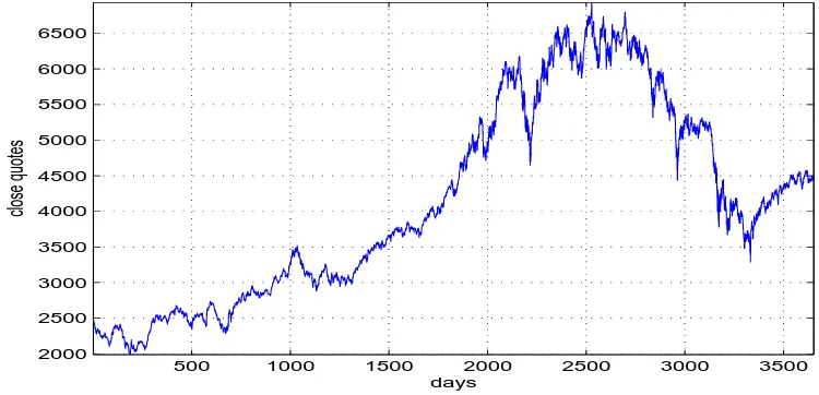
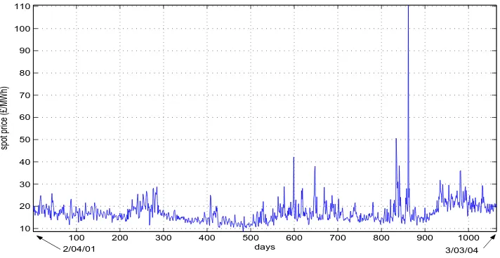
Electricity markets exhibit their own intrinsic complexities. There is a strong evidence of mean reversion and of spikes in spot prices, which in general are much more pronounced than in stock markets. The former can be observed by simple inspection of the data in both markets. Figure 1 shows daily closes of the FTSE100 index from 2/01/90 to 18/06/04. The nature of the price path can be seen as a combination of a deterministic trend together with random shocks. In contrast, Figure 2 shows that for electricity spot prices in England and Wales there is a strong mean reversion.3

This is, prices tend to oscillate or revert around a mean level, with extraordinary periods of volatility. These extraordinary periods of high volatility are reflected in the characteristic spikes observed in these markets.

500 1000 1500 2000 2500 3000 3500 2000

2500 3000 3500 4000 4500 5000 5500 6000 6500

days

close quotes

Figure 1: FTSE100 daily closes from 2/01/90 to 18/06/04.

3_{As proxy to daily closes of spot prices we have used the daily average of historical quoted}

100 200 300 400 500 600 700 800 900 1000 10

20 30 40 50 60 70 80 90 100 110

days

spot price (£/MWh)

2/04/01 3/03/04

Figure 2: Averaged daily prices in England and Wales from 2/04/01 to 3/03/04.

2.1

Normality Tests

In the Black-Scholes model prices are assumed to be log-normally distributed, which is equivalent to saying that the returns of the prices have a Gaussian or Normal dis-tribution.4 _{Although fat tails are observed in data from stock markets, indicating the}

probability of rare events being more frequent than predicted by a Normal distribu-tion, models based on this assumption have been largely used as a benchmark, albeit modified in order to account for fat tails.

For electricity though, the departure from Normality is more extreme. Figure 3 shows a Normality test for the electricity spot price from 2/04/01 to 3/03/04. If the returns were indeed Normally distributed the graph would be a straight line. We can clearly observe this is not the case, as evidenced from the fat tails. For instance, corresponding to a probability of 0.003 we have returns which are higher than 0.5; instead if the data were perfectly Normally distributed, the dotted lines suggests the probability of such returns should be virtually zero.

2.2

Deseasonalisation

One important assumption of the Black-Scholes model is that returns are assumed to be independently distributed. This can be easily evaluated with an autocorrelation test. If the data were in fact independently distributed, the correlation coefficient would be close to zero. A strong level of autocorrelation is evident in electricity

4_{Here we define “return” as in the classical definition; r}

t = ln(St+1/St). Note that this is also

−1.5 −1 −0.5 0 0.5 1 1.5 0.001

0.003 0.01 0.02 0.05 0.10 0.25 0.50 0.75 0.90 0.95 0.98 0.99 0.997 0.999

returns

probability

Figure 3: Normal probability test for returns of electricity prices from 2/04/01 to 3/03/04.

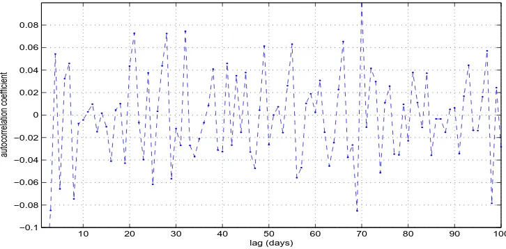
markets, as can be seen from Figure 4. As explained for instance in [15], the evidence of autocorrelation manifests an underlying seasonality. Furthermore, the lag of days between highly correlated points in the series reveals the nature of the seasonality. In this case, we may observe that the returns show significant correlation every 7 days (there is data for weekends also); which suggests some intra-week seasonality.

10 20 30 40 50 60 70 80 90 100

−0.2 −0.15 −0.1 −0.05 0 0.05 0.1 0.15 0.2 0.25

lag (days)

autocorrelation coefficient

7 14

21 28 35

42 49

56 63 70

77 84

91 98

Figure 4: Autocorrelation test for returns of electricity prices from 2/04/01 to 3/03/04.

a common approach which is to subtract the mean of every day across the series according to

Rt =rt−rd, (1)

whereRtis the defined deseasonalised return at timet, rt the return at timet andrd

is the corresponding mean (throughout the series) of the particular dayrtrepresents.

Figure 5 shows the autocorrelation test performed on the deseasonalised returns. As expected, the strong autocorrelation is no longer evidenced.

10 20 30 40 50 60 70 80 90 100

−0.1 −0.08 −0.06 −0.04 −0.02 0 0.02 0.04 0.06 0.08

lag (days)

autocorrelation coefficient

Figure 5: Autocorrelation test for deseasonalised returns of electricity prices.

2.3

Jumps

As seen from the Normality test, the existence of fat tails suggest the probability of rare events occurring is actually much higher than predicted by a Gaussian distribu-tion. By simple inspection of Figure 2 we can easily be convinced that the spikes in electricity data cannot be captured by simple Gaussian shocks.

We extract the jumps from the original series of returns by writing a numeri-cal algorithm that filters returns with absolute values greater than three times the standard deviation of the returns of the series at that specific iteration.5 _{On the}

second iteration, the standard deviation of the remaining series (stripped from the first filtered returns) is again calculated; those returns which are now greater than 3 times this last standard deviation are filtered again. The process is repeated until no

5_{As can be readily calculated, the probability in a Normal distribution of having returns greater}

further returns can be filtered. This algorithm allows us to estimate the cumulative frequency of jumps and other statistical information of relevance for calibrating the model.6

The relevance of the jumps in the electricity market is further demonstrated by comparing Figure 6 to Figure 3; where we can clearly observe that after stripping the returns from the jumps, the Normality test improves notoriously.

−0.3 −0.2 −0.1 0 0.1 0.2 0.3 0.001

0.003 0.01 0.02 0.05 0.10 0.25 0.50 0.75 0.90 0.95 0.98 0.99 0.997 0.999

returns

probability

Figure 6: Normal probability test for filtered returns of electricity prices.

6

3

The Model: Mean-reversion and Jump Diffusion

in the Electricity Spot

When modelling the electricity market two distinct approaches may be taken: mod-elling the spot market or modmod-elling the entire forward curve. As mentioned earlier, one of the appeals for using spot models relies on the fact that it is simple to in-corporate the observed characteristics of the electricity market. On the other hand, forward based models rely more heavily on the amount of historical data available. Since data of electricity prices in England and Wales is only regarded to be liquid and ‘well priced’ since the incorporation of NETA on March 27, 2001, the amount of data available is limited. This lack of sufficient data motivates the use of spot-based models rather than modelling the entire forward curve in the particular case of this market. It is worth emphasising that different power markets, although sim-ilar in some aspects, exhibit their own properties and characteristics. Hence, based on the manifest existence of mean-reversion and jumps on the data for England and Wales presented in the previous section, we propose a one-factor mean-reversion jump diffusion model; adjusted to incorporate seasonality effects.

Electricity can be bought in the spot market, but once purchased it must be used almost immediately, since in most cases electricity cannot be stored, at least not cheaply. Hedging strategies which typically involve holding certain amounts of the underlying (in this case electricity) are not possible, therefore in electricity markets forwards on the spot are typically used instead. As a consequence, it turns out it is extremely useful to be able to extract a closed-form formula for the forward curve from the spot-based model, which we are able to do for the model proposed here.

From the data analysis of the previous section we have concluded that two distinc-tive characteristics of electricity markets should be accounted for in the model; the mean reversion of the price and the sudden fluctuations in supply and low elasticity in demand which are reflected in price spikes. Moreover, it would also be important to incorporate some seasonality component which would be reflected in a varying long term level of mean reversion.

Schwartz [16] accounts for the mean reversion, and Luc´ıa and Schwartz [12] extend the mean reverting model to account for a deterministic seasonality. However, these models do not incorporate jumps. We propose in this paper a similar model extended to account for the observed jumps.

As in [12] let us assume that the log-price process, lnSt, can be written as

such that the spot price can be represented as

St =G(t)eYt (3)

whereG(t)≡eg(t) _{is a deterministic seasonality function andY}

tis a stochastic process

whose dynamics are given by

dYt=−αYtdt+σ(t)dZt+ lnJdqt. (4)

In (4) Yt is a zero level mean-reverting jump diffusion process for the underlying

electricity spot price St, α is the speed of mean reversion, σ(t) the time dependent

volatility,J the proportional random jump size, dZt is the increment of the standard

Brownian motion and dq a Poisson process such that

dqt=

1 with probabilityldt

0 with probability 1−ldt; (5)

where l is the intensity or frequency of the process.7 _{Moreover, J, dq}

t and dZt are

independent.

Regarding the jump size, J, the following assumptions are made:

• J is log-Normal, i.e. lnJ ∼N(µJ, σJ2).

• The risk introduced by the jumps is non-systematic and so diversifiable; fur-thermore, by assuming E[J] ≡ 1 we guarantee there is no excess reward for it.

With the assumptions made above, the properties of J can be summarised as follows:

J =eφ_{, φ∼N(−}σJ2 2 , σ

2

J); (6)

E[J] = 1; (7)

E[lnJ] =−σ 2 J

2 ; (8)

Var [lnJ] =σ2

J. (9)

Now, from (3) and (4) we can write the SDE for St, namely

dSt=α(ρ(t)−lnSt)Stdt+σ(t)StdZt+St(J −1)dqt, (10)

7_{Although the process followed byY}

tmean reverts around a zero level, it will be shown later that

where the time dependent mean reverting level is given by

ρ(t) = 1

α

dg(t)

dt +

1 2σ

2_(t)

+g(t). (11)

The interpretation of (10) is as follows. Most of the time dqt = 0, so we simply

have the mean reverting diffusion process. At random times however, St will jump

from the previous value St− to the new value JS_t−. Therefore the term S_t−(J −1)

gives us the change after and before the jump, ∆St=JSt−−St−.

3.1

Forward Price

The price at timetof the forward expiring at timeT is obtained as the expected value of the spot price at expiry under an equivalentQ-martingale measure, conditional on the information set available up to time t; namely

F(t, T) =EQt [ST|Ft]. (12)

Thus, we need to integrate first the SDE in (10) in order to extract ST and later

calculate the expectation.

For the first task we define the log-return as x≡ lnSt and apply Itˆo’s Lemma to

(10) to arrive at

dxt =α(µ(t)−xt)dt+σ(t)dZt+ lnJdqt, (13)

where

µ(t) = 1

α dg

dt +g(t) (14)

is the time dependent mean reverting level which depends on the seasonality function.

Regarding the expectation, we must calculate it under an equivalentQ-martingale measure. In a complete market this measure is unique, ensuring only one arbitrage-free price of the forward. However, in incomplete markets (such as the electricity market) this measure is not unique, thus we are left with the difficult task of se-lecting an appropriate measure for the particular market in question. Yet another approach, common in the literature, is simply to assume that we are already under an equivalent measure, and thus proceed to perform the pricing directly. This latter approach would rely however in calibrating the model through implied parameters from a liquid market. This is certainly difficult to do in young markets, as in the market of electricity in England and Wales, where there is no liquidity of instruments which would enable us to do this.

We follow instead Luc´ıa and Schwartz’ approach in [12], which consists of incor-porating a market price of risk in the drift, such that ˆµ(t)≡µ(t)−λ∗ _{and λ}∗ _≡λσ(t)

where λ denotes the market price of risk per unit risk linked to the state variable

xt. This market price of risk, to be calibrated from market information, pins down

the choice of one particular martingale measure. Under this measure we may then rewrite the stochastic process in (13) forxt as

dxt=α(ˆµ(t)−xt)dt+σ(t)dZˆt+ lnJdqt, (15)

where

ˆ

µ(t) = 1

α dg

dt +g(t)−λ σ(t)

α (16)

and dZˆt is the increment of a Brownian motion in the Q-measure specified by the

choice of λ.8

In order to integrate the process we multiply (15) by a suitable integrating factor and integrate between times t and T to arrive at

xT = g(T) + (xt−g(t))e−α(T−t)−λ Z T

t

σ(s)e−α(T−s)ds

+

Z T

t

σ(s)e−α(T−s)dZˆs+ Z T

t

e−α(T−s)lnJdqs. (17)

Now, since ST =exT, we can replace (17) into (12) to obtain

F(t, T) = Et[ST|Ft]

= ˆλTtG(T)

S(t)

G(t)

e−α(T−t)

Et h

e

R

T t σ(s)e−

α₍T

−s)_dZˆs

|FtiEt h

e

R

T t e−

α₍T

−s)_{lnJ dq}s

|Fti

= ˆλTtG(T)

S(t)

G(t)

e−α(T−t)

e12

R

T

t σ(s)2e−2

α(T₋s)_ds Et

h e

R

T t e−

α(T₋s)_{lnJ dqs}

|Fti (18)

where ˆλT t ≡ e

−λ

RT

t σ(s)e− α(T

−s)_ds

and expectations are taken under the risk-neutral measure. In Appendix C we prove that the expectation in (18) is

Et h

e

RT

t e− α(T

−s)ln_{J dq}s

|Fti = exp

Z T

t e−σ

2

J

2 e−

α(T

−s)+

σ2 J

2 e−2

α(T

−s)

lds−(T −t)l

. (19)

Finally, replacing ˆλT

t and (19) into (18) we obtain the price of the forward as

F(t, T) =G(T)

S(t)

G(t)

e−α(T−t)

e

R

T t [

1

2σ2(s)e−2

α(T₋s)_−λσ(s)e−α(T−s)]_ds+

R

T

t ξ(σJ,α,T,s)lds−l(T−t) ,

(20)

where ξ(σJ, α, T, s)≡e− σ2

J

2 e−

α(T

−s)+

σ2 J

2 e−2

α(T

−s)

.

8

4

Calibration

One of the arguments in favour of spot-based models is that they can provide a reliable description of the evolution of electricity prices. Moreover, these models are versatile in the sense that it is relatively simple to aggregate ‘characteristics’ to an existing family or class of models like for example adding a seasonality function. On the other hand, one of the drawbacks of these models is that it is quite difficult to estimate parameters given the relatively large number of parameters combined with a very small sample data, see for example [6], [10], [11].

One approach is to estimate all the parameters involved from historical data us-ing maximum likelihood estimators (MLE) through the approximations presented by Ball and Torous [2], [3].9 _{However, for the data of England and Wales this method}

yielded incorrect estimates, i.e. negative values for certain parameters that should otherwise be positive and estimates which depended heavily on the starting value of the parameters. We believe this is mainly due to the scarcity of data in this market.

As an alternative we propose a ‘hybrid’ approach that uses both historical spot data and forward market data. The former is used to calculate the seasonality com-ponent, the rolling historical volatility, the mean reversion rate and the frequency and standard deviation of the jumps.10 _{The latter is used to estimate the market price of}

risk.

4.1

Spot-based Estimates

4.1.1 Seasonality Function

In (3), G(t) is a deterministic function which accounts for the observed seasonality in power markets. The form of this seasonality function inevitably depends on the market in question. For instance, some electricity markets will exhibit a discernible pattern between summer and winter months. In such cases a sinusoidal function could be suitable (as suggested e.g. by Pilipovi´c in [14]). Other alternatives in-clude a constant piece-wise function, as for instance in [11]. Furthermore, Luc´ıa and Schwartz [12] introduce a deterministic function which discerns between weekdays and a monthly seasonal component.

However sophisticated these functions may be, they all rely on the inclusion of dummy variables and on being able to calibrate them correctly from the sample of

9

In these papers they demonstrate that for low values of the intensity parameter the Poisson process can be approximated by a Bernoulli distribution, such that the density function can be written as a mixture of Normals.

10_{By the restriction imposed in (7) we have reduced the need to calibrate the mean of the jumps}

historical data. As discussed earlier, this might be a serious constraint when dealing with markets with not enough historical data. Moreover, although it is reasonable to assume that there might be a distinguishable pattern between summer and winters in England and Wales, this is yet not evident from the available data.

Hence, including a seasonality function dependent on parameters to estimate from historical data would only add difficulty and unreliability to the already difficult cali-bration of the model. Instead, we have chosen to introduce a deterministic seasonality function which is a fit of the monthly averages of the available historical data with a Fourier series of order 5. In this way, we introduce a seasonality component into the model, but do not accentuate even further the problems involved in the calibration.11

The seasonality function is shown in Figure 7.

Jan Feb Mar Apr May Jun Jul Aug Sep Oct Nov Dec 15

15.5 16 16.5 17 17.5 18 18.5 19 19.5 20

average price (£/MWh)

monthly average Fourier fit

Figure 7: Seasonality function based on historical averaged months.

4.1.2 Rolling Historical Volatility

It can easily be shown that volatility is not constant across time in electricity markets. One common approach then, is to use as an estimate a rolling (or moving) historical volatility, as described in [10] for instance. In this case, we use a yearly averaged rolling historical volatility with a window of 30 days.

11

4.1.3 Mean reversion rate

The mean reversion is usually estimated using linear regression. In this case we regressed the increments of the returns ∆xt versus the series of returnsxt of the spot

price.

4.1.4 Jump Parameters

In order to estimate the parameters of the jump component of the spot dynamics, we filtered the data of returns using the code that was previously explained in Section 2.3. As an output of the code, we estimated the standard deviation of the jumps,

σJ, and the frequency of the jumps,l, which is defined as the total number of jumps

divided by the annualised number of observations.

4.2

Forward-based Estimate

We estimate the remaining parameter, the market price of risk λ, by minimising the square distances of the theoretical forward curve for different maturities (obtained through (20)) to given market prices of equal maturities.12

4.3

Results

The results obtained are summarised in the following table:

σJ l α λ(%)

0.67 8.58 1.18 (1.12, 1.24) 0.38 (0.37, 0.41)

Table 1: Annualised estimates for the standard deviation of the jumpsσJ, frequency

of the jumpsl, mean reversion rateαand market price of riskλ. When available, the 95% confidence bounds are presented in parenthesis.

Based on the result obtained for the standard deviation of the jumps through the filtering process discussed previously we could not conclude that the relationship imposed in the model between the mean and the variance of the logarithm of the jumps (through (8) and (9)) holds in each iteration. However, as mentioned earlier, this condition can be easily relaxed. This would lead, nonetheless, to the inclusion of an extra parameter to be estimated (the mean of the logarithm of the jumps). At this point, one must compromise between the imposed assumptions and the feasibility of calibrating a model dependent on too many parameters. The estimated frequency of

12_{The market quotes in reference were obtained from “Argus” and represent forward prices at}

jumps suggests that there are between 8 and 9 jumps per year, which is in agreement with observed historical data.

The estimated mean reversion rate represents a daily estimate. To interpret what the estimated value of mean reversion implies, let us re-write (15) in an Euler discre-tised form in a period ∆t where no random shocks or jumps have occurred, namely

xt+1 =α(ˆµ(t)−xt)∆t+xt. (21)

We may easily see that when we multiply the daily estimate by the appropriate annualisation factor (in this case 365), and since ∆t = 1/365; when α = 1 we have

xt+1 = ˆµ(t).

This is, whenα= 1 the process mean reverts to its equilibrium level over the next time step. In our case, the estimated parameter suggests it mean reverts very rapidly, in 0.84 days, this is, almost in a day. This is not surprising in electricity markets, and may already be inferred by the nature of the spot price series, as seen in Figure (2).

Escribano et al. and Knittel et al. in [1] and [11] respectively have extensively calibrated mean reverting jump diffusion models to electricity data for different mar-kets. In both cases, they calibrate discrete-time parameters. The connection between the time continuous parameters and the discrete version can be seen by writing the MRJD process defined in (15) as

xt =θt+βxt−1+ηt, (22)

where

θt ≡µˆ(t) 1−e−α

and β ≡e−α, (23)

and ηt represents the integral of the Brownian motion and the jump component

between times t−1 and t.

From (23) we may recover the discrete-time parameter corresponding to the mean reversion rate, which givesβ = 0.31; which is such that|β|<1, guaranteeing that the process mean reverts back to its non-constant mean. Moreover, our estimate of β is slightly lower (which in turn implies a higher mean reversion rate) than the estimates presented in [1] and [11] for different markets; thus revealing that the mean reversion of prices in the electricity market of England and Wales occurs more rapidly.

5

Applications

Pricing a European call option on a forward was first addressed by Black in 1976. Based solely on arbitrage arguments one can obtain the price of a forward contract under a GBM very easily, simple arguments then lead to a closed-form solution for a call option written on a forward, which is widely known as Black’s formula.13

However, when departing from the very idealised GBM, and incorporating both mean reversion and jump-diffusion to the process; closed-form solutions are very hard, if possible at all, to obtain. Duffie, Pan and Singleton in [8] are able to extract semi-closed-form solutions provided that the underlying follows an affine jump-diffusion (AJD); which they define basically as a jump-diffusion process in which the drift vec-tor, instantaneous covariance matrix and jump intensities all have affine dependence on the state vector.

On the other hand, without imposing these dependencies, a closed-form analytical solution might prove significantly harder to obtain. Hence, the pricing of these models is generally done numerically. Regardless of the numerical method employed, ulti-mately the performance of the model relies on the capability of successfully capturing the discussed characteristics of this market.

For instance, the model (once calibrated) must yield price paths for the price of electricity which resemble those observed in the market. In Figure 8 we show a simu-lated random walk which results from discretising (13) and later recovering the spot price asSt=ext; subject to the calibration discussed in the preceding section.14 Here

we observe that the price path succeeds in capturing the mean reversion and incor-porating the jumps, which are mostly (as desired) upwards. Moreover, the monthly averages of the simulated price path closely resembles the seasonality function, which is evidence that the process is mean reverting towards a time-dependent equilibrium level dictated mainly by the seasonality function, as expected from (14).

In order to further test the validity of the model, we show in Figure 9 the cali-brated forward curve with its 95% confidence interval, the averaged months from the calibrated forward curve and the monthly market forwards. We can observe that the forward curve sticks on average to levels close to the market curve; albeit showing a great degree of flexibility. By this we mean that the curve exhibits all the variety of shapes observed commonly in the market; which are commonly known as backwarda-tion (decrease in prices with maturity), contango (increase in prices with maturity) and seasonal (a combination of both).

13_{This derivation can be found in many textbooks, for a simple and intuitive explanation see e.g.}

[5].

14

In Figure 10 we show a forward surface for 5 months ahead. To understand this graph better, let us concentrate on the first month of July. For each day in June 2004 we calculate the forwards with starting date ti, i ∈ (1,30) with maturities Tk, k ∈ (1,31); where i sweeps across the days in June and k across maturities in July. The forward for each day in June then is calculated as the average of the forwards of maturityTk, thus reflecting the price of a forward contract of electricity for the entire

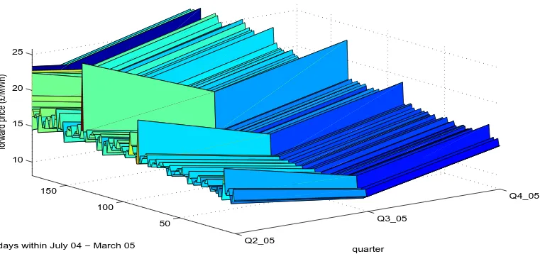
month of July, as quoted on the ith day of June. Similarly, in Figures 11 and 12 we show forward surface for quarters and seasons ahead.

As can be seen from Figure 10 for instance, the surface evolves in accordance to the monthly seasonalities, sticking to higher prices towards the end of the winter of 2004. This is again observed in Figure 11, where the prices for quarter 4, 2005 are higher, as expected. In Figure 12, we observe that for the second and third season ahead the calculated forward price exhibits little variation (seen as an almost straight line in the x-y plane). This is due to the fact that these are long-term contracts and the shocks become insignificant as maturity increases.

50 100 150 200 250 300 350 5

10 15 20 25 30 35 40 45 50

Simulated and calibrated electricity price for one year

days

spot price (£/MWh)

spot price seasonality monthly average

Figure 8: Simulated price path.

0 30 60 90 120 150 180

18 19 20 21 22 23 24 25 26 27 28

maturity (in days)

forward price (£/MWh)

July

August

September October

November

10 20

30 14 16 18 20 22 24 26

month days within June

forward price (£/MWh)

Figure 10: 5-months ahead forward prices for each day in June ‘04.

Q2_05

Q3_05

Q4_05 50

100 150

10 15 20 25

quarter days within July 04 − March 05

forward price (£/MWh)

W04−05

S05

W05−06

S06 20

40 60 80 10 15 20 25

month days within July 04 − September 04

forward price (£/MWh)

6

Conclusions

In the present paper we have analysed electricity spot prices in the market of England and Wales. The introduction of NETA changed in a fundamental way the behaviour of this market introducing competition and price variations. However, its implemen-tation only took place in March 27, 2001, resulting in not enough data, as of to day, to estimate or test models. Driven by this lack of data we proposed a spot-based model from which we can also extract in closed-form the forward curve. We then use both historical spot data as well as market forwards data to calibrate the parameters of the model.

Regarding the calibration of the model, we have circumvented a known drawback in electricity spot-based models, which is the overwhelming dependence on a great number of parameters to estimate. As the market evolves and more data becomes available (or possibly when using high-frequency data, thus extending the data-set) it will be possible to estimate all the parameters more robustly; as already pointed out by some papers which have analysed more mature markets. In the meantime, we have reduced the number of parameters to be estimated in the model. In doing so, we have used a ‘hybrid’ approach which combines estimating some parameters from historical spot data and the remaining from market forward prices. It can be argued that this is an arbitrary choice, since calibrating to a market curve starting at a different point might yield different parameters. Even if this were the case, this is not a serious flaw. This would imply re-calibrating the forward curve with respect to a different market curve. In a dynamic hedging-strategy this could be done as many times as necessary, depending on the exposure and the nature of the contract.

As to the output of the model, the simulated price path resembles accurately the evolution of electricity spot prices as observed in this market. With regards to the forward curve shown, it succeeds in capturing changing convexities, which is a serious flaw in models that fail to incorporate seasonality or enough factors. Moreover, as seen from the months-ahead forward surface for instance, the forward monthly prices increase with maturity until the end of the year, in accordance with market forward quotes.

A

Proof of Expected Value in Forward Equation

We want to evaluate

Et h

e

RT

t e− α(T

−s)ln_Jsdqs

i

=_Et h

e

RT

t αsdqs i

, (A 1)

where

αs≡e−α(T−s)lnJs. (A 2)

We will first calculate (A 1) in the interval [0, t] to later extend the calculation to the interval [t, T].

Let us start by defining Lt such that

Lt ≡ e

Rt

0αsdqs

≡ emt

, (A 3)

where mt is then

mt= Z t

0

αsdqs. (A 4)

and equivalently

dmt=αtdqt. (A 5)

In order to write the SDE followed by Lt for the process defined in (A 5) we

need to generalize Itˆo’s Lemma in order to incorporate the jumps. We will use the generalisation followed by Etheridge in [9] to write the SDE followed by Lt as15

dLt=

∂Lt(mt−)

∂mt

dmt−

∂Lt(mt−)

∂mt

(mt−mt−)dq+ (Lt−L_t−)dq, (A 6)

where we have not included any second derivative since the process defined by (A 5) is only a pure jump process.

In order to evaluate (A 6) let us first clarify the notation. If there is a jump in

{mt}t>0 it is of size αt and such that

mt=mt−+αt; (A 7)

where if a jump takes place at time t, the time t−

indicates the time interval just before the jump has occurred.

15

Hence by (A 4) we can also write (A 7) as

mt= Z t

0

αsdqs= Z t−

0

αsdqs+αt. (A 8)

Using (A 7) we can rewrite (A 3) as

Lt = emt

= emt−+αt

= Lt−e

αt

. (A 9)

Noting that ∂Lt(mt−)

∂mt =Lt− and replacing back (A 5), (A 7) and (A 9) into (A 6)

we get

dLt=Lt−(e

αt

−1)dqt; (A 10)

which we can integrate between 0 andt to obtain

Lt= 1 + Z t

0

Ls(eαs −1)dqs, (A 11)

where we have used that L0 = 1.

By taking expectations to the above equation we arrive to

E0[Lt] = 1 + Z t

0 E

0[Ls] (E0[eαs]−1)lds, (A 12)

where we are using the fact that E0[dq] = ldt and l is the intensity of the Poisson

process as had been defined in (5).

Defining now E0[Lt]≡nt we can rewrite (A 12) as

nt = 1 + Z t

0

ns(E0[eαs]−1)lds, (A 13)

which we can differentiate with respect tot to obtain

dnt

dt =nt(E0[e αt

]−1)l (A 14)

Integrating now over the interval [0, t] we get

Z t

0 dnt

nt

=

Z t

0

Finally, upon integrating and noting thatn0 =L0 = 1 and replacing the definitions of nt and Lt we obtain

E0 h

e

R

t

0αsdqs

i

=e

R

t

0(E0[eαs]−1)lds. (A 16)

It is then straightforward to show that

Et h

e

R

T t αsdqs

i

= e

R

T t (E0[e

αs_]−1)lds

; (A 17)

which proves (A 1).

Alternatively we can show the result in the following way. Note that the process

Rt

0 lnJsdqsis a compound Poisson process, hence it is a L´evy process. Let Rt

0 lnJsdqs= Rt

0 dLs with moment generating function, based on the L´evy-Khintchine

representa-tion,

E[eθLt

] = elt(ΨlnJ(θ)−1)

, (A 18)

where ΨlnJ(θ) is the moment generating function of the jumps lnJ. It is a well

known fact that for a deterministic function f(t) and a L´evy process ˜Lt the moment

generating function of the process Rt

0 f(s)dL˜s, when it exists, is given by

E[eθ

R

t

0f(s)dL˜s] =e

R

t

0Ψ(f(s)θ)ds, (A 19)

where Ψ(θ) is the log-moment generating function of the L´evy process ˜Lt. Therefore

E[eθ

Rt

0e−

α(t

−s)ln_{J dq}

] =el

R

t

0(ΨlnJ(e− α₍t

−s)_θ)−1)ds

(A 20)

and by evaluating atθ = 1 delivers the desired result.

Evaluating the integral

In order to evaluate (A 17) we must calculate first the expected value of eαs

. Thus, from (A 2) we wish to calculate

E0[eαs] =E0 h

ee−α(T−s)_lnJs i

; (A 21)

and calling h(s) =e−α(T−s) _then

E0[eαs] = E0

eh(s) lnJs

= E0

eh(s)φ

since we had defined that the jumps J were drawn from a Normal distribution, and by requiring that E[J] = 1 we had that φ ∼ N(−σ2J

2 , σ 2

J), where σJ is the standard

deviation of the jumps.

Thus, (A 22) yields

E0[eαs] =e− σ2

J

2 h(s)+

σ2 J

2 h2(s), (A 23)

and therefore (A 17) becomes

Et h

e

R

T t αsdqs

i

= e

R

T t (E0[e

αs_]−1)lds

= exp

Z T

t e−σ

2

J

2 h(s)+

σ2 J

2 h2(s)lds−

Z T

t lds

= exp

Z T

t e−σ

2

J

2 e−

α(T₋s)₊σ2J

2 e−2

α(T₋s)

lds−l(T −t)

. (A 24)

References

[1] ´Alvaro Escribano, Juan Ignacio Pe˜na, and Pablo Villaplana. Modelling electricity prices: International evidence.Universidad Carlos III de Madrid – working paper 02-27, June 2002.

[2] Clifford A. Ball and Walter N. Torous. A simplified jump process for common stock returns. The Journal of Finance and Quantitative Analysis, 18(1):53–65, March 1983.

[3] Clifford A. Ball and Walter N. Torous. On jumps in common stock prices and their impact on call option pricing. The Journal of Finance, 40(1):155–173, March 1985.

[4] Fred E. Benth, Lars Ekeland, Ragnar Hauge, and Bjorn F. Nielsen. A note on arbitrage-free pricing of forward contracts in energy markets. Applied Mathe-matical Finance, 10(4):325–336, 2003.

[5] Tomas Bj¨ork. Arbritrage Theory in Continuous Time. Oxford University Press, second edition, 2004.

[6] Les Clewlow and Chris Strickland. Energy Derivatives, Pricing and Risk Man-agement. Lacima Publications, 2000.

[7] Les Clewlow, Chris Strickland, and Vince Kaminski. Extending mean-reversion jump diffusion. Energy Power Risk Management, Risk Waters Group, February 2001.

[8] Darrel Duffie, Jun Pan, and Kenneth Singleton. Transform analysis and asset pricing for affine jump-diffusions. Econometrica, 68(6):1343–1376, November 2000.

[9] Alison Etheridge. A Course in Financial Calculus. Cambridge University Press, first edition, 2002.

[10] Alexander Eydeland and Krzysztof Wolyniec. Energy and Power Risk Manage-ment. John Wiley & Sons, first edition, 2003.

[11] Christopher R. Knittel and Michael R. Roberts. An empirical examination of deregulated electricity prices. POWER working paper PWP-087, 2001.

[13] Robert C. Merton. Continuous-Time Finance. Blackwell, first revised edition, 2001.

[14] Dragana Pilipovi´c. Energy Risk, Valuing and Managing Energy Derivatives. Mc Graw-Hill, 1998.

[15] Robert S. Pindyck and Daniel L. Rubinfeld. Econometric Models and Economic Forecasts. McGraw-Hill, fourth edition, 1998.

[16] Eduardo S. Schwartz. The stochastic behavior of commodity prices: Implications for valuation and hedging. The Journal of Finance, 52(3):923–973, July 1997.

Pricing in Electricity Markets: a mean reverting

jump diffusion model with seasonality

´

Alvaro Cartea and Marcelo G. Figueroa

Birkbeck College, University of London

September 2, 2005

Abstract

In this paper we present a mean-reverting jump diffusion model for the elec-tricity spot price and derive the corresponding forward in closed-form. Based on historical spot data and forward data from England and Wales we calibrate the model and present months, quarters, and seasons–ahead forward surfaces.

Keywords: Energy derivatives, electricity, forward curve, forward surfaces.

1

Introduction

One of the key aspects towards a competitive market is deregulation. In most elec-tricity markets, this has however only occurred recently. Prior to this, price variations were often minimal and heavily controlled by regulators. In England and Wales in particular, prices were set by the Electricity Pool, where due to centralisation and inflexible arrangements prices failed to reflect falling costs and competition. Deregu-lation came by the recent introduction on March 27, 2001 of NETA (New Electricity Trade Arrangement), removing price controls and openly encouraging competition.

Price variations have increased significantly as a consequence of the introduction of competition, encouraging the pricing of a new breed of energy-based financial products to hedge the inherent risk, both physical and financial, in this market. Most of the

∗_{Email: a.cartea@bbk.ac.uk and m.figueroa@econ.bbk.ac.uk. First version, June 2004. We are}

current transactions of instruments in the electricity markets is carried out through bilateral contracts ahead of time although electricity is also traded on forward and futures markets and through power exchanges.

One of the most striking differences that singles out electricity markets is that elec-tricity is very difficult or too expensive to store, hence markets must be kept in balance on a second-by-second basis. In England and Wales, this is done by the National Grid Company which operates a balancing mechanism to ensure system security.1

More-over, although power markets may have certain similarities with other markets, they present intrinsic characteristics which distinguish them. Two distinctive features are present in energy markets in general, and are very evident in electricity markets in particular: the mean reverting nature of spot prices and the existence of jumps or spikes in the prices.

In stock markets, prices are allowed to evolve ‘freely’, but this is not true for electricity prices; these will generally gravitate around the cost of production. Under abnormal market conditions, price spreads are observed in the short run, but in the long run supply will be adjusted and prices will move towards the level dictated by the cost of production. This adjustment can be captured by mean-reverting processes, which in turn may be combined with jumps to account for the observed spikes.

Therefore, to price energy derivatives it is essential that the most important char-acteristics of the evolution of the spot, and consequently the forward, are captured. Several approaches may be taken, generally falling into two classes of models: spot-based models and forward-spot-based models. Spot models are appealing since they tend to be quite tractable and also allow for a good mathematical description of the prob-lem in question. Significant contributions have been made by Schwartz, in [17] for instance the author introduces an Ornstein-Uhlenbeck type of model which accounts for the mean reversion of prices, and in [13] Luc´ıa and Schwartz extend the range of these models to two-factor models which incorporate a deterministic seasonal com-ponent. On the other hand forward-based models have been used largely in the Nord Pool Market of the Scandinavian countries. These rely heavily, however, on a large data set, which is a limiting constraint in the case of England and Wales. Finally, it must also be pointed out that the choice of model may sometimes be driven by what kind of information is required. For example, pricing interruptible contracts would require a spot-based model while pricing Asian options on a basket of electricity monthly and seasonal forwards calls for forward-based models.

The spot models described in [17] and [13] capture the mean reverting nature of electricity prices, but they fail to account for the huge and non-negligible observed spikes in the market. A natural extension is then to incorporate a jump component

in the model. This class of jump-diffusion models was first introduced by Merton to model equity dynamics, [14]. Applying these jump-diffusion-type models in electricity is attractive since solutions for the pricing of European options are available in closed-form. Nevertheless, it fails to incorporate both mean reversion and jump diffusion at the same time. Clewlow and Strickland [8] describe an extension to Merton’s model which accounts for both the mean reversion and the jumps but they do not provide a closed-form solution for the forward. A similar model to the one we present, although not specific to the analysis of electricity spot prices, has been analysed in Benth, Ekeland, Hauge and Nielsen [4].

The main contribution of this paper is twofold. First, we present a model that captures the most important characteristics of electricity spot prices such as mean reversion, jumps and seasonality and calibrate the parameters to the England and Wales market. Second, since we are able to calculate an expression for the forward curve in closed-form and recognising the lack of sufficient data for robust parameter estimation, we estimate the model parameters exploiting the fact that we can use both historical spot data and current forward prices (using the closed-form expression for the forward).2

The remaining of this paper is structured as follows. In Section 2 we present data analysis to support the use of a model which incorporates both mean reversion and jumps. In Section 3 we present details of the spot model and derive in closed-form the expression for the forward curve. In Section 4 we discuss the calibration of the model to data from England and Wales. In Section 5 we present forward surfaces reflecting the months, quarters and seasons–ahead prices. Section 6 concludes.

2_{All data used in this project has been kindly provided by Oxford Economic Research Associates,}

2

Data Analysis

For over three decades most equity models have tried to ‘fix’ the main drawback from assuming Gaussian returns. A clear example is the wealth of literature that deals with stochastic volatility models, jump-diffusion and more recently, the use of L´evy processes. One of the main reasons to adopt these alternative models is that Gaussian shocks attach very little probability to large movements in the underlying that are, on the contrary, frequently observed in financial markets. In this section we will see that in electricity spot markets assuming Gaussian shocks to explain the evolution of the spot dynamics is even a poorer assumption than in equity markets.

Electricity markets exhibit their own intrinsic complexities. There is a strong evidence of mean reversion and of spikes in spot prices, which in general are much more pronounced than in stock markets. The former can be observed by simple inspection of the data in both markets. Figure 1 shows daily closes of the FTSE100 index from 2/01/90 to 18/06/04. The nature of the price path can be seen as a combination of a deterministic trend together with random shocks. In contrast, Figure 2 shows that for electricity spot prices in England and Wales there is a strong mean reversion.3

This is, prices tend to oscillate or revert around a mean level, with extraordinary periods of volatility. These extraordinary periods of high volatility are reflected in the characteristic spikes observed in these markets.

500 1000 1500 2000 2500 3000 3500 2000

2500 3000 3500 4000 4500 5000 5500 6000 6500

days

close quotes

Figure 1: FTSE100 daily closes from 2/01/90 to 18/06/04.

3_{As proxy to daily closes of spot prices we have used the daily average of historical quoted}

100 200 300 400 500 600 700 800 900 1000 10

20 30 40 50 60 70 80 90 100 110

days

spot price (£/MWh)

2/04/01 3/03/04

Figure 2: Averaged daily prices in England and Wales from 2/04/01 to 3/03/04.

2.1

Normality Tests

In the Black-Scholes model prices are assumed to be log-normally distributed, which is equivalent to saying that the returns of the prices have a Gaussian or Normal dis-tribution.4 _{Although fat tails are observed in data from stock markets, indicating the}

probability of rare events being more frequent than predicted by a Normal distribu-tion, models based on this assumption have been largely used as a benchmark, albeit modified in order to account for fat tails.

For electricity though, the departure from Normality is more extreme. Figure 3 shows a Normality test for the electricity spot price from 2/04/01 to 3/03/04. If the returns were indeed Normally distributed the graph would be a straight line. We can clearly observe this is not the case, as evidenced from the fat tails. For instance, corresponding to a probability of 0.003 we have returns which are higher than 0.5; instead if the data were perfectly Normally distributed, the dotted lines suggests the probability of such returns should be virtually zero.

2.2

Deseasonalisation

One important assumption of the Black-Scholes model is that returns are assumed to be independently distributed. This can be easily evaluated with an autocorrelation test. If the data were in fact independently distributed, the correlation coefficient would be close to zero. A strong level of autocorrelation is evident in electricity

4_{Here we define “return” as in the classical definition; r}

t = ln(St+1/St). Note that this is also

−1.5 −1 −0.5 0 0.5 1 1.5 0.001

0.003 0.01 0.02 0.05 0.10 0.25 0.50 0.75 0.90 0.95 0.98 0.99 0.997 0.999

returns

probability

Figure 3: Normal probability test for returns of electricity prices from 2/04/01 to 3/03/04.

markets, as can be seen from Figure 4. As explained for instance in [16], the evidence of autocorrelation manifests an underlying seasonality. Furthermore, the lag of days between highly correlated points in the series reveals the nature of the seasonality. In this case, we may observe that the returns show significant correlation every 7 days (there is data for weekends also); which suggests some intra-week seasonality.

In order to estimate the parameters of the model, we strip the returns from this seasonality. Although there are several ways of deseasonalising the data, we follow a common approach which is to subtract the mean of every day across the series according to

Rt =rt−rd, (1)

whereRtis the defined deseasonalised return at timet, rt the return at timet andrd is the corresponding mean (throughout the series) of the particular dayrtrepresents. Figure 5 shows the autocorrelation test performed on the deseasonalised returns. As expected, the strong autocorrelation is no longer evidenced.

2.3

Jumps

As seen from the Normality test, the existence of fat tails suggest the probability of rare events occurring is actually much higher than predicted by a Gaussian distribu-tion. By simple inspection of Figure 2 we can easily be convinced that the spikes in electricity data cannot be captured by simple Gaussian shocks.

10 20 30 40 50 60 70 80 90 100 −0.2

−0.15 −0.1 −0.05 0 0.05 0.1 0.15 0.2 0.25

lag (days)

autocorrelation coefficient

7 14

21 28 35

42 49

56 63 70

77 84

91 98

Figure 4: Autocorrelation test for returns of electricity prices from 2/04/01 to 3/03/04.

standard deviation of the returns of the series at that specific iteration.5 _{On the}

second iteration, the standard deviation of the remaining series (stripped from the first filtered returns) is again calculated; those returns which are now greater than 3 times this last standard deviation are filtered again. The process is repeated until no further returns can be filtered. This algorithm allows us to estimate the cumulative frequency of jumps and other statistical information of relevance for calibrating the model.6

The relevance of the jumps in the electricity market is further demonstrated by comparing Figure 6 to Figure 3; where we can clearly observe that after stripping the returns from the jumps, the Normality test improves notoriously.

5_{As can be readily calculated, the probability in a Normal distribution of having returns greater}

than 3 standard deviations is 0.0027.

10 20 30 40 50 60 70 80 90 100 −0.1

−0.08 −0.06 −0.04 −0.02 0 0.02 0.04 0.06 0.08

lag (days)

autocorrelation coefficient

Figure 5: Autocorrelation test for deseasonalised returns of electricity prices.

3

The Model: Mean-reversion and Jump Diffusion

in the Electricity Spot

When modelling the electricity market two distinct approaches may be taken: mod-elling the spot market or modmod-elling the entire forward curve. As mentioned earlier, one of the appeals for using spot models relies on the fact that it is simple to in-corporate the observed characteristics of the electricity market. On the other hand, forward based models rely more heavily on the amount of historical data available. Since data of electricity prices in England and Wales is only regarded to be liquid and ‘well priced’ since the incorporation of NETA on March 27, 2001, the amount of data available is limited. This lack of sufficient data motivates the use of spot-based models rather than modelling the entire forward curve in the particular case of this market. It is worth emphasising that different power markets, although sim-ilar in some aspects, exhibit their own properties and characteristics. Hence, based on the manifest existence of mean-reversion and jumps on the data for England and Wales presented in the previous section, we propose a one-factor mean-reversion jump diffusion model; adjusted to incorporate seasonality effects.

−0.3 −0.2 −0.1 0 0.1 0.2 0.3 0.001

0.003 0.01 0.02 0.05 0.10 0.25 0.50 0.75 0.90 0.95 0.98 0.99 0.997 0.999

returns

probability

Figure 6: Normal probability test for filtered returns of electricity prices.

from the spot-based model, which we are able to do for the model proposed here.

From the data analysis of the previous section we have concluded that two distinc-tive characteristics of electricity markets should be accounted for in the model; the mean reversion of the price and the sudden fluctuations in supply and low elasticity in demand which are reflected in price spikes. Moreover, it would also be important to incorporate some seasonality component which would be reflected in a varying long term level of mean reversion.

Schwartz [17] accounts for the mean reversion, and Luc´ıa and Schwartz [13] extend the mean reverting model to account for a deterministic seasonality. However, these models do not incorporate jumps. We propose in this paper a similar model extended to account for the observed jumps.

As in [13] let us assume that the log-price process, lnSt, can be written as

lnSt =g(t) +Yt, (2)

such that the spot price can be represented as

St =G(t)eYt (3)

whereG(t)≡eg(t) _{is a deterministic seasonality function andY}

tis a stochastic process whose dynamics are given by

In (4) Yt is a zero level mean-reverting jump diffusion process for the underlying electricity spot price St, α is the speed of mean reversion, σ(t) the time dependent volatility,J the proportional random jump size, dZt is the increment of the standard Brownian motion and dq a Poisson process such that

dqt=

½

1 with probabilityldt

0 with probability 1−ldt; (5)

where l is the intensity or frequency of the process.7 _{Moreover, J, dq}

t and dZt are independent.

Regarding the jump size, J, the following assumptions are made:

• J is log-Normal, i.e. lnJ ∼N(µJ, σJ2).

• The risk introduced by the jumps is non-systematic and so diversifiable; fur-thermore, by assuming E[J] ≡ 1 we guarantee there is no excess reward for it.

With the assumptions made above, the properties of J can be summarised as follows:

J =eφ_{, φ∼N(−}σ2 J

2 , σ2J); (6)

E[J] = 1; (7)

E[lnJ] = −σ2J

2 ; (8)

Var [lnJ] =σ_J2. (9)

Now, from (3) and (4) we can write the SDE for St, namely

dSt=α(ρ(t)−lnSt)Stdt+σ(t)StdZt+St(J −1)dqt, (10)

where the time dependent mean reverting level is given by

ρ(t) = 1

α

µ

dg(t)

dt +

1 2σ

2_(t)

¶

+g(t). (11)

The interpretation of (10) is as follows. Most of the time dqt = 0, so we simply have the mean reverting diffusion process. At random times however, St will jump from the previous value St− to the new value JS_t−. Therefore the term S_t−(J −1) gives us the change after and before the jump, ∆St=JSt−−S_t−.

7_{Although the process followed byY}

tmean reverts around a zero level, it will be shown later that

3.1

Forward Price

The price at timetof the forward expiring at timeT is obtained as the expected value of the spot price at expiry under an equivalentQ-martingale measure, conditional on the information set available up to time t; namely

F(t, T) =EQ

t [ST|Ft]. (12)

Thus, we need to integrate first the SDE in (10) in order to extract ST and later calculate the expectation.

For the first task we define xt ≡lnSt and apply Itˆo’s Lemma to (10) to arrive at

dxt =α(µ(t)−xt)dt+σ(t)dZt+ lnJdqt, (13)

where

µ(t) = 1

α dg

dt +g(t) (14)

is the time dependent mean reverting level which depends on the seasonality function.

Regarding the expectation, we must calculate it under an equivalentQ-martingale measure. In a complete market this measure is unique, ensuring only one arbitrage-free price of the forward. However, in incomplete markets (such as the electricity market) this measure is not unique, thus we are left with the difficult task of se-lecting an appropriate measure for the particular market in question. Yet another approach, common in the literature, is simply to assume that we are already under an equivalent measure, and thus proceed to perform the pricing directly. This latter approach would rely however in calibrating the model through implied parameters from a liquid market. This is certainly difficult to do in young markets, as in the market of electricity in England and Wales, where there is no liquidity of instruments which would enable us to do this.

We follow instead Luc´ıa and Schwartz’ approach in [13], which consists of incor-porating a market price of risk in the drift, such that ˆµ(t)≡µ(t)−λ∗ _{and λ}∗ _≡λσ(t)

α ; where λ denotes the market price of risk per unit risk linked to the state variable

xt. This market price of risk, to be calibrated from market information, pins down the choice of one particular martingale measure. Under this measure we may then rewrite the stochastic process in (13) forxt as

dxt=α(ˆµ(t)−xt)dt+σ(t)dZˆt+ lnJdqt, (15)

where

ˆ

µ(t) = 1

α dg

dt +g(t)−λ σ(t)

and dZˆt is the increment of a Brownian motion in the Q-measure specified by the choice of λ.8

In order to integrate the process we multiply (15) by a suitable integrating factor and integrate between times t and T to arrive at

xT = g(T) + (xt−g(t))e−α(T−t)−λ

Z _T

t

σ(s)e−α(T−s)ds

+

Z _T

t

σ(s)e−α(T−s)dZˆs+

Z _T

t

e−α(T−s)lnJdqs. (17)

Now, since ST =exT, we can replace (17) into (12) to obtain

F(t, T) = Et[ST|Ft]

= ˆλT tG(T)

µ

S(t)

G(t)

¶_e−α(T−t) Et

h

eRtTσ(s)e−α(T−s)dZˆs|F_t

i

Et

h

eRtTe−α(T−s)lnJdqs|F_t

i

= ˆλT tG(T)

µ

S(t)

G(t)

¶_e−α(T−t) e12

R_T

t σ(s)2e−2α(T−s)dsE_t

h

eRtTe−α(T−s)lnJdqs|F_t

i

(18)

where ˆλT

t ≡ e−λ

RT

t σ(s)e−α(T−s)ds and expectations are taken under the risk-neutral

measure. In Appendix C we prove that the expectation in (18) is

Et

h

eRtTe−α(T−s)lnJdqs|Ft

i

= exp

·Z _T

t

e−σ 2 J

2 e−α(T−s)+ σ_J2

2 e−2α(T−s)lds−(T −t)l

¸

. (19)

Finally, replacing ˆλT

t and (19) into (18) we obtain the price of the forward as

F(t, T) =G(T)

µ

S(t)

G(t)

¶_e−α(T−t)

eRtT[12σ2(s)e−2α(T−s)−λσ(s)e−α(T−s)]ds+ RT

t ξ(σJ,α,T,s)lds−l(T−s)_,

(20) where ξ(σJ, α, T, s)≡e−

σ2_J

2 e−α(T−s)+ σ_J2

2 e−2α(T−s).

8_{Although the market price of risk itself could be time-dependant, here we assume it constant}