STUDIES ON IMPROVING TEXTURE SEGMENTATION PERFORMANCE USING GENERALIZED GAUSSIAN MIXTURE MODEL INTEGRATING DCT AND LBP

ISSN: 1992-8645 www.jatit.org E-ISSN: 1817-3195

NEURAL NETWORK OPTIMIZATION USING

SHUFFLEDFROG ALGORITHM FOR SOFTWARE DEFECT

PREDICTION

1

REDDI. KIRAN KUMAR, 2S.V.ACHUTA RAO

1

Department of Computer Science, Krishna University, Machilipatnam, India- 521001

2

Research Scholar, Krishna University, Machilipatnam, India- 521001 E-mail: 1 [email protected], [email protected]

ABSTRACT

Software Defect Prediction (SDP) focuses on the detection of system modules such as files, methods, classes, components and so on which could potentially consist of a great amount of errors. SDP models refer to those that attempt to anticipate possible defects through test data. A relation is present among software metrics and the error disposition of the software. To resolve issues of classification, for the past many years, Neural Networks (NN) have been in use. The efficacy of such networks rely on the pattern of hidden layers as well as in the computation of the weights which link various nodes. Structural optimization is performed in order to increase the quality of the network frameworks, in two separate cases: The first is the typically utilized approximation error for the present data, and the second is the capacity of the network to absorb various issues of a general class of issues in a rapid manner along with excellent precision. The notion of Back Propagation (BP) is quite elementary; the result of neural networks is tested against the desired outcome. Genetic algorithms (GA) are a type of search algorithms built, based on the idea of natural evolution. A neural network using Shuffled Frog Algorithm for improving SDP is proposed.

Keywords:Software Defect Prediction (SDP), Neural Network (NN), Back Propagation (BP), Genetic Algorithm (GA) and Shuffled Frog Leaping Algorithm (SFLA)

1. INTRODUCTION

This Software Defect Prediction (SDP) holds an important place in the domain of software quality and dependability. Software faults may be defined as errors, mistakes or defects in computer programs or systems which lead to false or unusual outcomes, or leading the software to perform in unexpected ways. When a software module consists of too many flaws that gravely inhibit execution, it is said to be fault-prone. The procedure of identifying such faulty modules in a particular software is SDP. The conventional methods of discovering faults in a software are code review, unit testing, integration testing and system testing. But, when a particular software’s dimensions increase by way of the number of coding statements and complexity, the process of discovering as well as repairing errors becomes harder as well as costly with regard to computation; through the usage of advanced testing and evaluatory processes. Furthermore, Boehm gleaned that the discovery and repair of issues once a particular software has been delivered, is costlier, money and effort-wise, when

compared to repairing the fault in the initial phases of the life cycle of the software. Identification of fault-prone software modules allows professionals to focus their effort and capabilities on the problematic regions of the software under construction [1 & 2].

ISSN: 1992-8645 www.jatit.org E-ISSN: 1817-3195 hidden slab for the identification of features in the

mid-range of the information and a Gaussian complement is employed in a different hidden slab for the identification of characteristics for the upper and lower limits of the data. Hence, the outcome layer will receive dissimilar “views of the data”. Compounding the two characteristics sets in the outcome layer points to more accurate predictions. The other structure picked is the GRNN, which is a memory-based network that gives an estimation of continuous variables and comes together at the base (linear or non-linear) regression surface. As it is a one-pass learning algorithm possessing a very parallel architecture, the barest minimum of information in a multidimensional measurement environment; the algorithm allows for seamless movement from one ascertained value to the next.

Discovering the appropriate algorithm for the modeling of software elements to various stages of error severity is a crucial task [4].A model grounded in the Biological Neural Network, is the Artificial Neural Network (ANN) and is typically referred to as merely Neural Network. Artificial neurons, described as nodes are interlinked for the purpose of constructing ANNs. The structure of neural networks is crucial for the performance of a specific operation. Certain neurons are placed specifically for obtaining input from the external environment. Because they are not linked to one another, the structure of the neurons is as a layer, referred to as an input layer. The neurons present in the input layer provide certain output which functions as the input for the adjacent layer [5].

Two types of NN structures that may be combined are feed-forward networks and recurrent/recursive networks. Networks that possess completely linked layers, like the multi-layer perceptron, and networks with convolution and pooling layers are feed-forward networks. Every single network acts as a classifier, however each has a distinct strength of its own. Completely linked feed-forward NNs are non-linear learners which may, at the most, be utilized as an alternate to linear learners.

Because the network is non-linear and has the capacity to incorporate previously trained word embeddings, it results in exceptional classification precision. A set of studies achieved better syntactic parsing outcomes through the mere replacement of the linear model of the parser with a completely linked feed-forward neural network[6].The networks are initially directed to simulate the behaviour of active and passive circuits. These networks, now trained are called as neural network models. These may now be utilized in high level

simulation and designs, and are shown to produce the fastest and most precise responses to the task because of the information they acquired during the process of training

When compared to traditional approaches; such as numerical modeling techniques, that are exceptionally costly with regard to computation, or analytical techniques that could be hard to attain for newly obtained gadgets, or empirical modeling techniques which possess a large range and poor precision, neural networks prove to be more efficient and may be employed for a great number of applications as well as modeling techniques [7].

A three-layer feed-forward NN is proven to be capable of approximating a non-linear continuous function to a random precision. They are employed in plenty of fields like prediction, system modeling and control. Because of the specific structure, NNs are excellent in absorbing learning algorithms like Genetic Algorithm (GA) as well as Back Propagation. Typically, there are two learning stages for an NN: Firstly, a network architecture is determined with a specific set of inputs, hidden notes as well as outputs. Secondly, an algorithm is picked to execute the training procedure.

But, it is not a must for a stable architecture to give its best results during the learning stage. A small network might be incapable of performing well due to the restrictive processing potential. A big network, though, might possess repetitive links and the execution cost remains heavy. Both constructive and destructive algorithms may be utilized in order to attain the network architecture. Constructive algorithms begin with the small networks while the destructive algorithm begins with the big networks.

Hidden layers, nodes and links are later eliminated to compress the network in a dynamic manner. The pattern of a network architecture may be modeled as a search issue. Gas are used to achieve the results. Pattern-classification approaches may be seen designing networks [8].Fitness testing consumes too much time in various real-world applications of evolutionary calculation. A way to decrease the computation time is through the replacement of the fitness function with an approximate framework with lesser computational cost. These frameworks are called meta-models or substituted in optimization. A model for evolutionary optimization uses approximate models for applications in order to achieve optimization.

ISSN: 1992-8645 www.jatit.org E-ISSN: 1817-3195 manipulate the evolutionary procedure; that is, to

determine how frequently the approximate model ought to be utilized as opposed to the initial fitness function, to make sure of the merging of the evolutionary algorithm to the right optimum of the initial issue as well as to decrease calculation cost to the highest degree. The better the quality of the framework, it should replace the initial fitness function more frequently. The learning capacity of the NNs is especially crucial for the time online learning is required to be executed at the time of optimization.

Optimization of the structure of NNs is performed before they are used for the purpose of fitness testing in evolutionary pattern optimizations [9]. GAs are based on the evolution of people. In a certain environment, people who are more suited to it, are fit to survive and pass down their genes to future generations; and less adaptable humans die. The goal of GAs is to utilize basic representations to code complicated architectures and basic computations to better those architectures. GAs are hence, defined by their representations and operators.

In a GA, a single chromosome is correlated to a binary string. The bits in each string are named as genes and their changing values are alleles. A set of single chromosomes are a population. Fundamental genetic operators incorporate reproduction, crossover and mutation [10]. GAs and artificial NNs are methods for learning and optimization, which have been based on biological mechanisms. NNs utilize inductive learning and typically need samples, whereas GAs adopt deductive learning and need objective evaluation function.

This paper suggests neural network structure optimization using Shuffled Frog Algorithm. Section 2 deals with literature related to this work, section 3 reveals the methods used in the work, section 4 deals with results and discusses obtained results and finally section 5 concludes the work.

2. LITERATURE REVIEW

Yang et al., [11] researched this issue and proposed a network pruning algorithm grounded in sparse representation, called SRP. The suggested method begins with a sizeable network, extracted crucial hidden neurons from the initial architecture utilizing a forward selection criterion which lessens the residual output error. Additionally, the proposed algorithm possesses no restrictions of network kind. The efficacy of the suggested technique was tested on various benchmark data sets. The outcomes

reveal that SRP is more accurate as opposed to other methods.

Fan and Wen [12] proposed a novel mind evolutionary algorithm (MEA) grounded in the basic MEA model in order to optimize the NN’s architecture and weights, where like taxis and different operators of architecture optimization are planned. Using such taxis operators, the local optimum is discovered and then overshooting the constriction of local range by the usage of dissimilation operators, the global optimum is attained in the global solution environment. The outcomes of the simulations revealed that the approach was efficient and accurate.

Mohseni and Tan [13] suggested a novel mixed training algorithm comprising error back-propagation (EBP) as well as variable structure systems (VSS) for the optimization of parameter updating of NNs. In order to optimize the number of neurons in the hidden layer, a new term dependent on the outcome of the hidden layer is combined to the cost function as a penalty term so as to optimally utilize hidden blocks connected to weights correlating to every single block in the hidden layer. Additionally, apart from analysing the imposed dynamics of the EBP method, the global reliability of the mixed training methodology and restrictions on the design variables were observed. The suggested method has plenty of benefits including assured convergence, increased strength as well as decreased sensitivity to preliminary weights of the network.

Shahriari-kahkeshi and Askari [14] proposed the plan of a recurrent neural network (RNN) trained Shuffled Frog Leaping Algorithm (SFLA) for the purpose of identifying and following control of non-linear continuous stirred tank reactors (CSTR). RNNs were applied to approximate unknown dynamic systems and SFLAs were employed for the training and optimization of connection weights of the RNNs. The suggested control design used neural control system synthesis was employed in the closed-loop control system for accurate control inputs. The outcomes revealed that the RNN-SFLA controllers have extraordinary dynamic responses and also that they adapted excellently to changes.

ISSN: 1992-8645 www.jatit.org E-ISSN: 1817-3195 that the novel WNN algorithm has improved

convergence rate, positioning accuracy, favourable application prospects and future research value.

Yu et al., [16] utilized SFLA as a basis for NNs in speech emotion detection. SFLA is utilized to train arbitrary preliminary information, optimize link weights and thresholds of NNS with rapid network convergence speech. Outcomes revealed that the SFLA network shows excellent detection rate in the field.

Ye et al., [17] used the SFLA with pseudo code and flow charts to ease its execution. The researches utilized SFLA to optimize weight and threshold value of BP networks. Experimental results revealed that SFLA outperformed GA in optimizing BP networks’ weight and threshold values that are utilized in non-linear function fitting.

Che et al., [18] proposed a brilliant technique of swarm neural networks (SNN) for dealing with equalities-constrained non-convex optimization issues. The suggested technique dealt with the issue in two sections that compound local searching capacity of one-layer RNN and global searching capacities of SFLA. Firstly, an RNN framework grounded in typical non-convex optimization was issued. Also, dependent on the SFLA model, NNs are considered as frogs that ought to be split into many memeplexes and develop individual differential equations in order to find an accurate local solution. And lastly, numerical samples with outcomes are provided to display the efficacy and excellent features of the suggested method resolving non-convex optimization issues.

3. METHODOLOGY

In this section, we discuss neural network utilizing BP, neural network using GA and proposed neural network using SFLA.

3.1. Neural Network using Back Propagation

A BPNN learns by utilizing the generalized delta rule in a two phase propagate-adapt cycle. The first randomly drawn weights are applied to the NN in order to create a starting point in which to initiate the search. During the starting point, approximates are compared with the expected outcome, and an error is calculated for each of the observations. The error for the first observation is computed by decreasing an amount equal to the estimated value from the true value. Total of the squared errors is typically utilized as objective function [19].

One of the most commonly used NN algorithms is BP and it may divided into four

major stages. After choosing the weights of the network arbitrarily, the BP algorithm is utilized to calculate the required rectifications. The algorithm may be divided into the below mentioned four steps [20]:

i) Feed-forward computation

ii) Back propagation to the output layer

iii) Back propagation to the hidden layer

iv) Weight updates

The best technique for carrying out supervised learning is the BP algorithm. BP has been employed in many learning tasks and has come out as the standard algorithm for the training of multi-layer perceptron networks. BP is grounded in gradient descent as it is q conjugate gradient. It typically utilizes a least-square optimality criterion, determining a technique for computing the gradient of the error specifically for the weights for a certain input, through the propagation of the error backwards through the network. Error BP is essentially a search procedure that tries to decrease a whole network error function like the sum E of the squared error of the network output over an ensemble of training input/output pairs:

(

)

1

1

2

m

j j

j

E

t

o

=

=

_∑

−

where

t

o

The back propagation algorithm determines two sweeps of the network: firstly, a forward sweep from the input layer to the output layer, and next, a backward sweep from the output to the input layer. In the first stage, input vectors are propagated through the network to give outputs of the network. The backward step is alike to the forward one, except that error values calculated, are propagated back through the network, so as to evaluate how the weights ought to be altered during the training phase. The fundamental process for the BP algorithm is reported in Figure 1.

ISSN: 1992-8645 www.jatit.org E-ISSN: 1817-3195 Initialize network weights randomly

termination condition

Assign as net input to each unit in the input layer its corresponing element in the input vector. The output for each unit is its ne

while not do

t input Calculate network output by forwarding input signals in the network Calculate the error of each output neuron

all hidden neurons calculate weights updates propagate the error back through th

for do

e network.

Update weights of the network.

end for

end while

Figure 1: Pseudo code of the Back Propagation algorithm

3.2. Neural Network Using Genetic Algorithm

Genetic Algorithms is a way of approaching machine learning by appropriating behaviour of the human gene as well as Darwin’s theory of natural selection. GA is a part of Evolutionary Algorithms which provide solutions depending on the methods more generally discovered in nature like mutation, selection, crossover etc.

Genetic Algorithms are applied starting with an individual population that is typically represented in the form of trees. A probable solution is represented by each tree or say chromosome in this case. Nodes on the tree denote certain traits that relate to the issue for which the solution is being searched. Collectively, the set of possible solutions to the problem is (represented by the chromosomes) as known as the population [22].

GA’s appear in the picture when it is required to solve issues which can have various solutions. Here, genetic algorithms are utilized to cluster the classes delineated according to object oriented metrics into subsystems or typically called components of software. As described earlier, GA utilizes an approach similar to Darwin’s “Survival of the Fittest” theory or natural selection. Why this approach is being deliberated upon is due to the large solutions set that provides a many possible solutions to an issue.

When employing a GA in a problem, a couple of implications are made. They are mentioned below

• A fitness function must be present for evaluating if a solution is a possible or not

• When a solution is found, a representation of it must be made by a chromosome.

• Which genetic operators will be employed must be decided.

Furthermore the definition of a solution in this case would be one which would be both complete as well as valid. In terms of a representation, it may be assumed that the possible solutions have been encoded in the solutions space.

The GA is a search technique grounded in the idea of evolution, and particularly with the notion of the survival of the fittest. The usage of GA on NNs make a hybrid neural network where the weights of the neural network are computed through GA method. From all the search spaces of the probable weights, the GA will create new points of the probable solution.

The first stage to compute its values, is to delineate the solution field with a genetic representation (problem encoding) as well as a fitness function to define the better solutions. These two components of a GA are the only problem dependent on the GA method. When initial populations of elements (genotype or chromosomes) have been generated, the method s utilized by these algorithms in order to reach a solution to the issue are connected to evolutionary theories:

i. Selection → few chromosomes of the current population are chosen for the breeding of a new generation. A small set is chosen arbitrarily and the remaining are chosen based on how they suit a fitness function.

ii. Genetic operations → when the initial chromosomes have been delineated by those that fit more appropriately with the fitness function, the remaining population will be built through genetic operations. Fatnesses of the new chromosomes will additionally, be verified and compared to the worst chromosomes of the previous generation to determine who remains in the population. Mutation: Altering one or more gens of few chromosomes of the entire set & Crossover: Crossing two or more chromosomes in the set amongst themselves.

A pseudo-code for Genetic algorithm is [23]:

(

)

( )

( )

1. Creation of the initial population

2. while !solution

a Evaluate the fitness of all the chromosomes of the population

b The best chromosomes will be selected to reproduce, using

mut

( )

ation and crossover.

c Substitute the worsts chromosomes of the previous generation

by the new produced chromosomes.

ISSN: 1992-8645 www.jatit.org E-ISSN: 1817-3195 Genetic algorithms are algorithms for

optimizing and machine learning grounded loosely in many features of biological evolution. They require five components [24]:

i. A method of coding solutions to the problem on chromosomes.

ii. An evaluation function which returns a rating for each chromosome given to it. iii. A method to initializing the population of

chromosomes.

iv. Operators that may be applied to parents when they reproduce to alter their genetic composition. Standard operators are mutation and crossover.

v. Parameter settings for algorithms, operators etc.

3.3. Proposed Neural Network Using Shuffled Frog Algorithm

ANN technology, inspired by neurobiological (the brain’s structure) theories of massive interconnection and parallelism, is perfect for undertakings like pattern recognition and discrimination. One of the first researchers to extend the application of neural networks into optimization was Hopfield (1984), and it has been successfully applied to a variety of combinatorial optimization problems. The ANN learns to solve a problem by developing a memory capable of associating a large number of input parameters with a resulting set of outputs or effects. The ANN develops a solution system by training using examples given to it [25].

SFLA is a meta heuristic for solving optimization problems. SFLA is a cooperative search metaphor that is population based and is occasioned by natural memetics. Memetic evolution by way of influencing ideas from one individual to the next in a local search is employed by the algorithm. Theoretically, this is alike to Particle Swarm Optimization (PSO). A shuffling technique allows for the exchange of data amongst local searches, thereby attaining global optimum [26].

In the SFLA, the population comprises of frogs of like structures. Every frog denoted one solution. The total population is split into various subgroups. Different subgroups may be considered as different frog memes. Every subgroup attempts a local search. They can correspond with one another and better their memes among local units. Once a pre-determined number of memetic evolution stages are done, data is transferred between memeplexes in a shuffling manner. This shuffling

makes sure that the cultural evolution in the direction of any specific interest is completely unbiased. The local search and the shuffling procedures alternate till the stopping criteria is satisfied. [27].

The SFLA is based on observing, imitating, and modeling the behavior of a number of frogs during the process of searching for the location that possesses the most amount of available food. The primary benefit of SFLA is its fast convergence speed. The SFL Emerges the benefits of both the genetic-based memetic algorithm (MA) and the social behavior-based PSO algorithm.

SFLA is a population based arbitrary search algorithm occasioned from nature meme tics. In the SFLA, a set of possible solutions determined by a set of frogs that is divided into several communities known as memplexes. Every frog in the memeplexes performs a local search. Inside of each memeplex, the single frog’s behavior may be influenced by other frogs and evolution through a procedure of memtic evolution will occur. After a particular number of memetic evolution stages, the memeplexes are pressured to join together and novel memeplexes are developed through a shuffling process.

The flowchart of Shuffled frog leaping algorithm is illustrated in Fig. 1.The various steps are as follows:

1. The SFLAincludes a population ‘P’ of possible solutions, determined by a set of virtual frogs(n).

2. Frogs are arranged in descending order as pe their fitness and then divided into subsets called as memeplexes (m).

3. Frogs i is expressed as

(

)

i i1 i2 is

X = X , X ,....X where S represents number of variables.

4. Within each memeplex, the frog with worst and best fitness are identified as

w

X and

X

X g .

6. The frog with worst fitness is improved according to the following equation.

( )

( )

i b w

n e w w o l d w i m a x i m a x

D = r a n d ( ) X - X

X = X + D - D ≤ D ≤ D

where rand is an arbitrary number in the range of [0,1];D is the frog leaping step size of _i

ISSN: 1992-8645 www.jatit.org E-ISSN: 1817-3195 change in a frog’s position. If the fitness value of

new X_w is better than the current one, Xw will be

accepted. If it isn’t improved, then the calculated are repeated with

b

X replaced by X g . If there is

no possibility of improvement in the case, a new

w

X will be generated arbitrarily. Reiterate the update operation for a certain number of iterations [28].The flowchart of SFLA is given below in Figure 3:

Figure 3: Flowchart Of SFLA

4. RESULTS&DISCUSSION

In this section, the classification accuracy, precision, recall and F measure are evaluated from table 1 to 4 and figure 4 to 7.

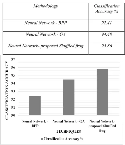
Table 1: Classification Accuracy

Methodology Classification Accuracy %

Neural Network - BPP 92.41

Neural Network - GA 94.48

Neural Network- proposed Shuffled frog 95.86

Figure 4: Classification Accuracy

From table 1 and figure 4, it is observed that the Neural Network method improved classification accuracy by 2.22%, 1.45% and 3.66% when compared with the BPP, GA and proposed Shuffled frog methods.

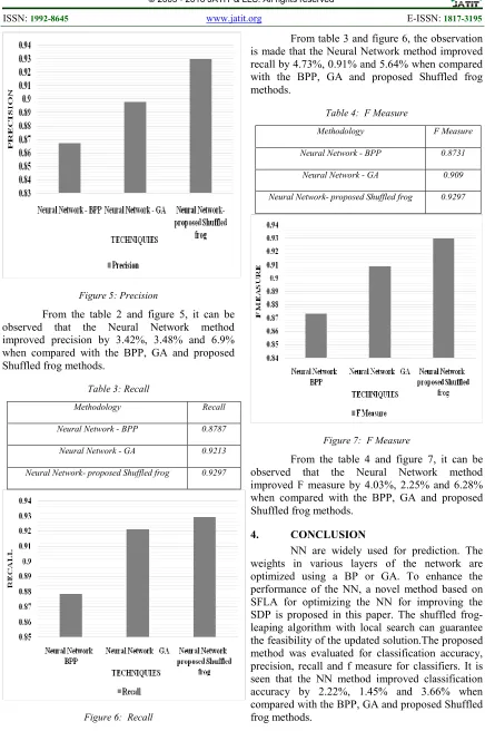
Table 2: Precision

Methodology Precision

Neural Network - BPP 0.8677

Neural Network - GA 0.8979

Neural Network- proposed Shuffled frog 0.9297 Start

Initialize parameters: Population size (P) Number of memeplexes (m) Number of Iterations within each

memeplex

Generate random population of P solutions (frogs), Calculate fitness of

each individual

frog

Sorting population in descending order of their fitness

Divide P solutions into m memeplexes

Local search

Shuffle evolved memeplexes

Determine the best solution Termination=true

End

No

ISSN: 1992-8645 www.jatit.org E-ISSN: 1817-3195

Figure 5: Precision

From the table 2 and figure 5, it can be observed that the Neural Network method improved precision by 3.42%, 3.48% and 6.9% when compared with the BPP, GA and proposed Shuffled frog methods.

Table 3: Recall

Methodology Recall

Neural Network - BPP 0.8787

Neural Network - GA 0.9213

Neural Network- proposed Shuffled frog 0.9297

Figure 6: Recall

From table 3 and figure 6, the observation is made that the Neural Network method improved recall by 4.73%, 0.91% and 5.64% when compared with the BPP, GA and proposed Shuffled frog methods.

Table 4: F Measure

Methodology F Measure

Neural Network - BPP 0.8731

Neural Network - GA 0.909

Neural Network- proposed Shuffled frog 0.9297

Figure 7: F Measure

From the table 4 and figure 7, it can be observed that the Neural Network method improved F measure by 4.03%, 2.25% and 6.28% when compared with the BPP, GA and proposed Shuffled frog methods.

4. CONCLUSION

ISSN: 1992-8645 www.jatit.org E-ISSN: 1817-3195

REFRENCES:

[1]. Prasad, M. C., Florence, L., & Arya, A. (2015). A Study on Software Metrics based Software Defect Prediction using Data Mining and Machine Learning Techniques. International Journal of Database Theory and Application, 8(3), 179-190.

[2]. Gayathri, M., & Sudha, A. (2014). Software Defect Prediction System using Multilayer Perceptron Neural Network with Data Mining. International Journal of Recent Technology and Engineering (IJRTE) ISSN, 2277-3878. [3]. Thwin, M. M. T., & Quah, T. S. (2005).

Application of neural networks for software quality prediction using object-oriented metrics. Journal of systems and software, 76(2), 147-156.

[4]. Sandhu, P. S., Lata, S., & Grewal, D. K. (2012). Neural Network Approach for Software Defect Prediction Based on Quantitative and Qualitative Factors. International Journal of Computer Theory and Engineering, 4(2), 298.

[5]. Panchal, G., Ganatra, A., Shah, P., & Panchal, D. (2011). Determination of over-learning and over-fitting problem in back propagation neural network.International Journal on Soft Computing, 2(2), 40-51.

[6]. Goldberg, Y. (2015). A Primer on Neural Network Models for Natural Language Processing. arXiv preprint arXiv:1510.00726. [7]. Chakraborty, M. (2012). Artificial neural

network for performance modeling and optimization of CMOS analog circuits. arXiv preprint arXiv:1212.0215.

[8]. Leung, F. H., Lam, H. K., Ling, S. H., & Tam, P. K. (2003). Tuning of the structure and parameters of a neural network using an improved genetic algorithm. Neural Networks, IEEE Transactions on, 14(1), 79-88.

[9]. Hüsken, M., Jin, Y., & Sendhoff, B. (2005). Structure optimization of neural networks for evolutionary design optimization. Soft Computing, 9(1), 21-28.

[10]. Vishwakarma, M. D. D. (2012). Genetic Algorithm based Weights Optimization of Artificial Neural Network. International Journal of Advanced Research in Electrical, Electronics and Instrumentation Engineering, 1(3), 206-211.

[11]. Yang, J., Ma, J., Berryman, M., & Perez, P. (2014, July). A structure optimization algorithm of neural networks for large-scale data sets. In Fuzzy Systems (FUZZ-IEEE), 2014 IEEE International Conference on (pp. 956-961). IEEE.

[12]. Fan, T., & Wen, R. (2009, March). MEA for Designing Neural Network Weights and Structure Optimization. In Computer Science and Information Engineering, 2009 WRI World Congress on (Vol. 6, pp. 111-115). IEEE. [13]. Mohseni, S. A., & Tan, A. H. (2012).

Optimization of neural networks using variable structure systems. Systems, Man, and Cybernetics, Part B: Cybernetics, IEEE Transactions on, 42(6), 1645-1653.

[14]. Shahriari-kahkeshi, M., & Askari, J. (2011, December). Nonlinear continuous stirred tank reactor (CSTR) identification and control using recurrent neural network trained Shuffled Frog Leaping Algorithm. In Control, Instrumentation and Automation (ICCIA), 2011 2nd International Conference on (pp. 485-489). IEEE.

[15]. Feng, H., Rui-Yu, L., Li, Z., & Li, Z. (2009, December). Application of shuffled frog leaping algorithm and wavelet neural network in sound source location. In Information Science and Engineering (ICISE), 2009 1st International Conference on (pp. 3600-3604). IEEE.

[16]. Yu, H., Huang, C., Jin, Y., & Zhao, L. (2010, October). Automatic recognition of speech emotion using Shuffled Frog Leaping Algorithm. In Image and Signal Processing (CISP), 2010 3rd International Congress on (Vol. 7, pp. 3505-3508). IEEE.

[17]. Ye, H., Yang, L., & Liu, X. (2013, September). Optimizing weight and threshold of BP neural network using SFLA: applications to nonlinear function fitting. In 2013 Fourth International Conference on Emerging Intelligent Data and Web Technologies (pp. 211-214). IEEE.

[18]. Che, H., Li, C., He, X., & Huang, T. (2015). An intelligent method of swarm neural networks for equalities-constrained nonconvex optimization.Neurocomputing.

ISSN: 1992-8645 www.jatit.org E-ISSN: 1817-3195 [20]. Cilimkovic, M. Neural Networks and Back

Propagation Algorithm. Institute of Technology Blanchardstown, Blanchardstown Road North Dublin, 15.

[21]. Azzini, A. (2005). A New Genetic Approach for Neural Network Design and Optimization (Doctoral dissertation, Tesi di dottorato, Universita degli Studi di Milano). [22]. Rawat, M. S., & Dubey, S. K. (2012).

Software defect prediction models for quality improvement: a literature study. International Journal of Computer Science, 9, 288-296. [23]. Perez, S. (2008). Apply genetic algorithm

to the learning phase of a neural network. [24]. Montana, D. J. (1995). Neural network

weight selection using genetic lgorithms. Intelligent Hybrid Systems, 8(6), 12-19.

[25]. Eusuff, M., Lansey, K., & Pasha, F. (2006). Shuffled frog-leaping algorithm: a memetic meta-heuristic for discrete optimization. Engineering Optimization, 38(2), 129-154.

[26]. Pourmahmood, M., Akbari, M. E., & Mohammadpour, A. (2011). An efficient modified shuffled frog leaping optimization algorithm. Int. J. Comput. Appl, 32(1), 0975-8887.

[27]. Lu, K., Ting, L., Keming, W., Hanbing, Z., Makoto, T., & Bin, Y. (2015). An Improved Shuffled Frog-Leaping Algorithm for Flexible

Job Shop Scheduling

Problem. Algorithms, 8(1), 19-31.