4188
COMPUTER SIMULATION OF LARGE DISPLACEMENTS OF
THERMOELASTIC RODS
1BAISAROVA G., 2BRZHANOV R., 3KIKVIDZE O.G., 4LAKHNO V., 5BURIACHOK V.,
6CHUBAIEVSKYI V.
1Department of Construction Engineering of the Caspian State University of Technology and Engineering
named after Sh. Yesenov, Aktau, Republic of Kazakhstan
2Department of Construction Engineering of the Caspian State University of Technology and Engineering
named after Sh. Yesenov, Aktau, Republic of Kazakhstan
3President of the Georgian Mechanical Union Full professor of Akaki Tsereteli State University, Kutaisi,
Georgia
4Department of Construction Engineering of the Caspian State University of Technology and Engineering
named after Sh. Yesenov, Aktau, Republic of Kazakhstan
5Department of Information and Cybersecurity, Borys Grinchenko Kyiv University, Ukraine 6Kyiv National University of Trade and Economics, Kyiv, Ukraine
E-mail: 1[email protected], 2[email protected], 3 [email protected], 4[email protected], 5[email protected], 6[email protected]
ABSTRACT
This paper presents the results of research, including elements of theoretical calculation, computer simulation and experimental study of displacements, internal force factors and temperature fields during plane deformation of rods. The temperature problem for a bar of rectangular cross section was studied. The differential equation of one-dimensional unsteady heat conduction is solved in the Mathcad system for boundary conditions of the first and third kind, including for non-stationary boundary conditions established experimentally. The results of numerical calculations in Mathcad are in good agreement with the results of the experiment. The maximum error is 17% at the end of heating at
t
=440 с. The coordinates of the reduced center of gravity with uneven temperature distribution are determined. It has been established that an increase in the temperature gradient affects the coordinates of the reduced center of gravity and, in fact, does not depend on the law of temperature change. The calculations were carried out in the Mathcad system. The simulation experiments carried out in the Mathcad system reduced the laboriousness of work by about 20% to study factors that influence internal stresses and temperature fields during plane deformation of rods.Keywords:Thermoplastic Rod, Computer Simulation, Non-Stationary Thermal Conductivity
1.INTRODUCTION
Rods, as structural elements, are widely used in building structures, machines, measuring devices, robots and manipulators as force elements, mechanical energy accumulators, elastic transmission mechanisms, flexible couplings, etc. Therefore, the study of the laws of deformation is necessary for solving practically important problems.
The reliability of building structures, machines and devices depends on the reliability of structural elements and, accordingly, on the accuracy of their calculations. Therefore, at the present stage, the requirements for accuracy of
calculations have increased significantly, taking into account the real properties of the material and the loading mode. For such situations at the initial stages of research, it is better to use mathematical packages, for example, Mathcad.
4189 change the shape, for alloys with a shape memory, the displacements of the elastic line can be comparable with the geometric dimensions of the rod in the temperature range of thermoelastic martensitic transformations.
Solving a non-linear problem gives the opportunity to investigate the stability of the elements of engineering and building structures, establish a critical load and study for critical behavior, and it is rather difficult to perform this study without the use of modern application software packages, which predetermined the relevance of our research topic.
2. ANALYSIS OF LITERARY DATA AND
PROBLEM STATEMENT
In the works [1–3] large displacements of flexible rods under mechanical loads are studied, but the authors refer to the results of calculations performed manually and it is difficult to establish the adequacy of these calculations. In these works, it is assumed that the length of the elastic line does not change, i.e. there is a neutral layer where the deformation is zero. However, as the temperature changes, all layers of the rod are deformed due to temperature expansion, which is not always taken into account by the developers of specialized software.
In the works [4–6] the methods for calculating nonlinear deformation of rods under thermomechanical loading are considered. The complex development of the authors, in particular, took into account the geometric characteristics of the rods, but the results of computer modeling were not supported by the publications of the authors.
All of the foregoing has led to the relevance of our study, in which the emphasis is placed on presenting the results of computer simulation in the Mathcad system of the results of calculations of non-linear problems of rod deformation under thermomechanical loading [7–11].
Statement of work – is to develop methods for calculating nonlinear problems of deforming rods under thermomechanical loading using the Mathcad system.
To achieve the goal, the following tasks were set and solved:
- the non-stationary problem of heat conduction for the rod was investigated using the mathematical editor Mathcad;
- the generalized geometric characteristics of a flat section were also studied with non-uniform
heating and a variable modulus of elasticity of the material;
- the nonlinear boundary value problem of plane bending of the rod under thermomechanical loading was formulated;
- a numerical integration of nonlinear equations was carried out using the Mathcad package.
3.METHODS AND MODELS
The calculation of the temperature distribution for each structural element requires the compilation of a heat balance equation. In the case of dependence of the heat distribution in the body both on the coordinates and on time, we have a non-stationary mode of thermal conductivity.
Unsteady heat conduction mode takes place during various technological operations.
The heat equation (Fourier equation) in Cartesian coordinates has the following form:
Q
c
x
T
y
T
z
T
a
t
T
1
)
(
22
2 2
2 2
(1)
where
c
– the heat capacity of the solid,T
– temperature,a
/(
c
)
– coefficient of thermal diffusivity,
– the density of the material,
- thermal conductivity of a solid,Q
– density of internal heat sources.The boundary conditions of the first kind, when the temperature is set on the limiting body surfaces. In the general case, the temperature at the boundary may depend on the coordinates of the boundary points and time.
.
)
,
,
,
(
)
,
,
,
(
;
)
,
,
,
(
)
,
,
,
(
;
)
,
,
,
(
)
,
,
,
(
;
0
, 0 3
, 0
, 0 2
, 0
, 0 1
, 0
b x b x
h y h y
l z l
z
t
z
y
x
T
t
z
y
x
T
t
z
y
x
T
t
z
y
x
T
t
z
y
x
T
t
z
y
x
T
t
(2)
4190 surface as a function of time and coordinates of surface points.
The boundary conditions of the third kind, in which the heat flux is assumed to be proportional to the temperature difference between the surface and the environment [12–14].
;
]
)
,
,
,
(
[
]
)
,
,
,
(
[
;
0
, 0 , 0 b x f b xT
t
z
y
x
T
x
t
z
y
x
T
t
;
]
)
,
,
,
(
[
]
)
,
,
,
(
[
;
0
, 0 , 0 h y f h yT
t
z
y
x
T
y
t
z
y
x
T
t
.
]
)
,
,
,
(
[
]
)
,
,
,
(
[
;
0
, 0 , 0 l z f l zT
t
z
y
x
T
z
t
z
y
x
T
t
(3)The boundary conditions of the fourth kind (conjugation conditions), which are reduced to the simultaneous specification of the equality of temperatures and heat fluxes at the interface, when the problem of heat exchange between two media (solid-liquid, body-body, liquid-liquid) is solved, in each of which the transfer heat is described by the equation:
,
2 1T
грT
.
2 2 1 1 грn
T
n
T
(4)The one-dimensional problem of unsteady heat conduction is being solved for boundary conditions of the first and third kind. The equations and the corresponding boundary conditions are specified. The problem of one-dimensional unsteady thermal conductivity.
The temperature field varies by coordinate
y
and by timet
,
T
T
(
y
,
t
)
, source of heat in the bodyQ
0
. In this case, equation (4) is simplified and takes the form:
t
T
a
y
T
1
2 2 (5)For the heat equation and third kind boundary conditions in the similarity theory, dimensionless combinations were obtained representing the Fourier similarity criterion (Fo) for the differential heat and bio equation (Bi) for the boundary condition [15, 16]:
2 *
h
t
a
Fo
,
h
Bi
(6)where
t
*– is a characteristic heating time.For the numerical solution of these equations, dimensionless quantities are involved, and the partial differential equation is solved in the Mathcad system for different boundary conditions.
h
y
y
t
t
t
T
T
T
f
;
;
*, (7)
where
t
* – the final value of temporary heating.When the boundary conditions of the first kind are specified for the temperature, the functional dependence is used which is established by us experimentally. Then a study of the problem for the boundary condition of the third kind is carried out. The boundary and initial conditions in dimensionless quantities have the form (two variants are presented):
),
(
,
0
,
0
;
1
,
1
,
)
0
(
,
0
,
0
1 1t
f
T
y
t
T
y
f
T
y
t
).
(
,
0
,
0
;
1
,
1
,
1
,
0
,
0
1t
f
T
y
t
T
y
T
y
t
(8)For excessive dimensionless temperature, in the absence of a heat source (
Q
0
), equation (5) has the form:4191 where:
/
T
f .
The boundary condition of the third kind for excessive dimensionless temperature.
.
Bi
y
(10)For numerical integration in partial derivatives in the Mathcad system, the built-in pdesolve function is used.
4.RESULTS OF COMPUTATIONAL
EXPERIMENTS IN THE MATHCAD SYSTEM.
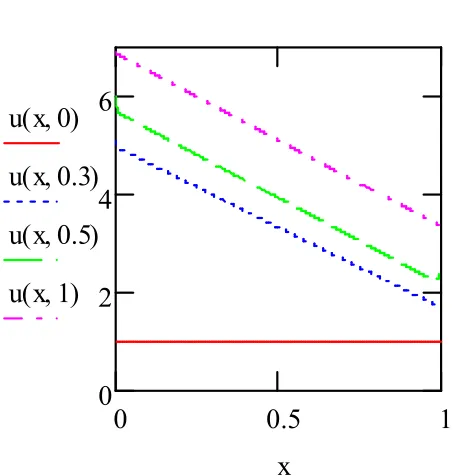
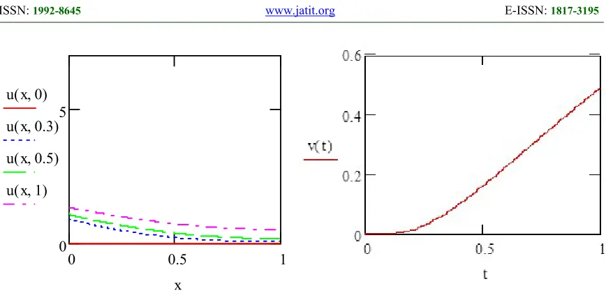
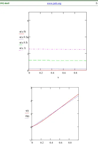
In this section of the article, the results of the calculation are shown, from which it can be seen that the theoretical conclusions are inconsistent with the experiment. The maximum difference is observed at the end of heating, with somewhere around eight minutes of heating and the maximum error is 17% for this point. And for the main part, in general, good agreement between theory and experiment.
0
0.5
1
0
2
4
6
u x 0
(
)
u x 0.3
(
)
u x 0.5
(
)
u x 1
(
)
[image:4.612.187.414.283.521.2]x
4192
0
0.5
1
0
5
u x 0
(
)
u x 0.3
(
)
u x 0.5
(
)
u x 1
(
)
x
f f
f f
T t
T T
y
T t
T t
f y
929 . 23 153
. 0 , 1
; 878 . 24 688
. 20 ) ( , 0
98 . 0 98 . 0
322 . 0 322 . 0 1
[image:5.612.91.525.71.286.2]
Figure 2: Solution of the problem under the third kind boundary conditions of Bio criterion Bi=0.185, u(x,t)=(T-Tf )/Тf dimensionless excess temperature of Fourier criterion
4193
0 0.2 0.4 0.6 0.8
0 2 4 6
u x 0( ) u x 0.1( ) u x 0.5( ) u x 1( )
x
0 0.2 0.4 0.6 0.8 1
0 1 2 3
v t( ) f1t( )
[image:6.612.116.460.67.579.2]t
Figure 3: Solution of the problem under the boundary conditions of the third kind on both boundaries. Heat transfer coefficients on the heating surface α1=79.5 and on the free surface α=7.95f1(t) – experimental results
In the course of research, the generalized geometric characteristics of a flat section are studied taking into account the variable elastic parameter with an uneven temperature distribution.
We considered some flat section in the coordinate system
xoy
and wrote down the following integrals:
A
x
yF
x
y
dA
S
*(
,
)
, *(
,
)
,
F
y
xF
x
y
dA
S
4194 where
F
(
x
,
y
)
– scalar function that describes the state of the elementary material area and the form of which depends on the material model.In formulas (11) integration is carried out over the entire area. Magnitudes
S
x* andS
*y are called generalized static moments about axesx
and
y
respectively.With a parallel transfer of the axes, the values of the generalized static moments are changed:
,
,
* * *1 * * *
1
S
bA
S
S
aA
S
x
x
y
y
(12) wherea
– distance between parallel axesy
and1
y
,b
– distance between parallel axesx
and1
x
,
A
dA
y
x
F
A
*(
,
)
(13)a generalized flat section area is represented.
To select the axes х1 and у1 so that Sх1*=0 и
Sу1*=0. Then the coordinates of the reduced center of gravity of a flat section are determined by using the formulas [16, 17]:
,
/
,
/
* * **
A
x
S
A
S
y
c
x c
y (14)where
S
x*,
S
*y
generalized static moments about axesx
andy
respectively.Therefore, in order to determine the coordinates of the reduced center of gravity of a flat section, it is necessary in an arbitrary coordinate system
xoy
to calculate the generalized static moments and the generalized area of a flat section. It is easily seen that for a homogeneous body with homogeneous structural parameters, the generalized geometric characteristics of a flat section are geometric characteristics, and the reduced center of gravity coincides with the center of gravity (geometric center).We considered the generalized moments of inertia of a flat section about the axes
x
andy
:,
)
,
(
,
)
,
(
,
)
,
(
* 2
* 2
*
A
xy A
y A
x
dA
y
x
xyF
I
dA
y
x
F
x
I
dA
y
x
F
y
I
(15)
where
I
*x,
I
*y
generalized moments of inertiaabout axes
x
,
y
respectively,I
*xy
generalized centrifugal moment.)
,
(
)
(
)
,
(
x
y
E
T
E
x
y
F
(16)
)
(
)
(
0 k kS
k
T
T
E
T
E
, (17)where
k,
T
S,
k
– constant values,T
S– initial temperature,T
current temperature.n
h
y
T
T
T
T
0
(
1
0)(
/
)
. (18)In this part
T
0 andT
1 temperature cross section aty
0
andy
h
respectively.
.
)]
(
/
1
[
/
/
]
)]
(
/
1
[
[
0 0
0 0
h hk k S k
k k S k
C
T
T
E
dy
dy
T
T
E
y
y
(19)
4195
),
/(
),
/(
,
/
,
/
3 0 * * 0 * *dh
E
I
I
dh
E
A
A
T
T
T
h
y
y
x x S
.
2
;
1
],
1
)
/
/[(
)
/
1
(
0 *
k
T
T
E
E
k S F F k
Then,
1 0 * * * 2 * * 1 0 * 2 * 1 0 * 1 0 *.
)]
1
(
1
[
,
,
)]
1
(
1
[
,
)]
1
(
1
[
)]]
1
(
1
[
[
y
d
T
A
A
y
I
I
y
d
T
y
I
y
d
T
T
y
d
y
y
k k c x xc k k x k k k k c
(20) Numerical calculation was carried out for thefollowing values of constants:
.
1
,
1
,
34
,
108
,
26
0 1 0 00
C
T
C
T
C
k
n
T
SAs a result of the calculation, the values of the reduced geometric characteristics of a flat section are obtained:
.
973
.
0
,
081
.
0
,
328
.
0
,
504
.
0
* * *
A
I
I
y
Xc x CIn this chapter, a numerical study of generalized geometric characteristics and a reduced center of gravity are carried out. And calculations were carried out for two cases: when the elastic modulus changes (decreases) by 5% and when the elastic modulus changes (decreases) by 10%, under the same conditions. And calculations were carried out for two cases: when the elastic modulus changes (decreases) by 5% and when the elastic modulus changes (decreases) by 10%, under the same conditions 2500 С. But for magnesium alloys, for aluminum
alloys, etc., for other materials these changes amount to 11%–30%.
[image:8.612.84.549.58.601.2]And the calculations show that up to 5% in principle, the usual geometric characteristics can be used, but when the elastic modulus decreases by 10% or more, it is necessary to use generalized geometric characteristics and it is necessary to calculate the stress-strain state using these characteristics.
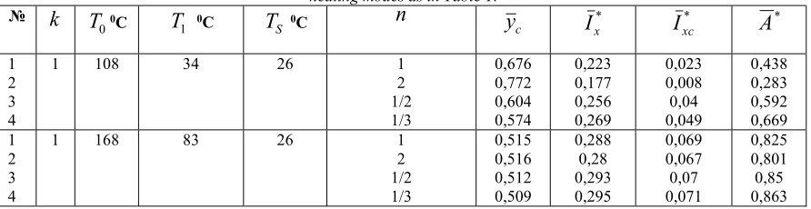
Table 1: Calculation data with a decrease in the elastic modulus of 5%
№
k
0
T
0С
1
T
0СS
T
0Сn
c
y
*x
I
*xc
I
A
*1 2 3 4
1 108 34 26 1
2 1/2 1/3 0,504 0,504 0,503 0,502 0,328 0,326 0,33 0,33 0,081 0,081 0,082 0,082 0,973 0,965 0,98 0,984 1 2 3 4
1 168 83 26 1
2 1/2 1/3 0,507 0,507 0,505 0,504 0,31 0,307 0,313 0,314 0,076 0,075 0,077 0,077 0,913 0,9 0,925 0,931
Table 2: Calculation data with a decrease in the elastic modulus of 10% with the same heating modes as in Table 1.
№
k
0
T
0С1
T
0СS
T
0Сn
c
y
*x
I
*xc
I
A
*1 2 3 4
1 108 34 26 1
2 1/2 1/3 0,676 0,772 0,604 0,574 0,223 0,177 0,256 0,269 0,023 0,008 0,04 0,049 0,438 0,283 0,592 0,669 1 2 3 4
1 168 83 26 1
[image:8.612.84.530.617.732.2]4196 From the calculation results given in Tables 1 and 2, it can be seen that with a slight (up to 5%) change in the elastic modulus of the material, the reduced center of gravity actually coincides with the geometric center and the form of the function of temperature variation in the cross section slightly influences the position of the reduced center of gravity. When the elastic modulus changes by 10% at the same temperature conditions, the coordinate of the reduced center of gravity does not coincide with the geometric center. The coordinate of the reduced center of gravity substantially depends on the heating temperatures of the upper and lower faces of the cross section and on the law of temperature variation in the cross section.
The nonlinear problem of deformation of the rod under thermomechanical loading is also being considered. The radius of curvature of the thermoelastic line before and after deformation through 0and and the angle of inclination of the tangent thermoelastic line to the z axis before and after deformation through 0 and respectively, moving along the z axis through w, and along the y axis through v. It is apparent that
w=w(l),v=v(l),=(l),=(l), the arc l–length of deformed thermoelastic line (related coordinate) or, w=w(l0),v=v(l0),=(l0),=(l0), where l0 – is the length of the arc undeformed thermoelastic line.
The system of equations for curved rods:
dv/dl0=(1+0)sin– sin0,
dw/dl0=(1+0)cos– cos0,
d/dl0=(1+0)/0+
x,dM/dl0=(1+0)(Hsin– Rcos –m),
dR/dl0= – (1+0 )qy,
dH/dl0= – (1+0 )qz,
N=Hcos + Rsin.
(21)
From these equations, the differential equation for the straight bars can be obtained, at 0=0 and 0 equations bending straight bars are obtained.
The system of equations for straight rods:
,
,
1
cos
)
1
(
,
sin
)
1
(
0 0
x
dz
d
dz
dw
dz
dv
dM/dz=(1+0)(Hsin-Rcos –m)
dR/dz= – (1+0 )qy,
dH/dz= – (1+0 )qz.
(22)
These equations constitute a closed system that describes the plane bending of a straight rod under thermomechanical loading.
In [5,6, 8, 15, 16, 18] boundary conditions for different types of edge fixing were formulated.
The method of numerical solution of a nonlinear boundary value problem: for the numerical calculation, the following dimensionless quantities are introduced:
L
T
T
T
h
y
y
L
q
M
M
L
q
m
m
L
q
H
H
L
q
R
R
L
L
w
w
L
v
v
L
l
l
f x x
,
,
,
,
,
,
,
,
,
,
2 *
* *
*
(23)
L
z
z
( for straight rods),L
l
l
00
,* , ,
q
q
q
yz
yz ,where
L
– the length of the rod to deformation,*
q
– the maximum value of the distributed load.4197
)
cos
sin
)(
1
(
,
)
1
(
,
)
1
(
,
1
,
cos
cos
)
1
(
,
sin
sin
)
1
(
0 0 0 0 0 0 0 0 0 0 0 0 0 0 0m
R
H
l
d
M
d
q
l
d
H
d
q
l
d
R
d
l
d
d
l
d
w
d
l
d
v
d
z y x
(24 ),
sin
cos
R
H
N
(25),
)
1
(
1 0 * *
E
T
y
d
y
I
h
T
L
q
I
M
x f x x
(26)).
)
1
(
(
1
1 0 2 2 *0
q
T
E
T
d
y
L
h
N
A
f
(27)
Similarly, the equations in dimensionless quantities can be written to describe the deformation of straight rods.
)
cos
sin
)(
1
(
,
)
1
(
,
)
1
(
,
,
1
cos
)
1
(
,
sin
)
1
(
0 0 0 0 0m
R
H
z
d
M
d
q
z
d
H
d
q
z
d
R
d
z
d
d
z
d
w
d
z
d
v
d
z y x
(28)We solve a number of problems of nonlinear deformation of a straight rod of rectangular cross section. Define displacements and internal force factors for different values of mechanical load and non-uniform heating within elastic limits. The temperature varies only along the height of the cross section according to a given law. In the basic equations, the dimensionless quantities are chosen in such a way that characterizing the maximum values of external loads
q
* and material parameters were concentrated in the motion parameterq
.
For numerical integration of vector
Y
the following components are presented:,
)
,
,
,
,
,
(
Y
1Y
2Y
3Y
4Y
5Y
6 TY
(29)where
,
,
,
,
,
,
2 3 4 5 61
v
Y
Y
w
Y
R
Y
M
Y
H
Y
(30). the following components are presented:
.
3
.
0
,
56
,
30
,
26
,
7
.
0
,
024
.
0
,
012
.
0
0 0 0
n
C
T
C
T
C
T
L
d
h
h a fFor a given material and geometric dimensions of the beam
q
*
14
,
4
q
кН/м. Load vector does not change direction [18–23].The boundary conditions at the left end correspond to the second condition, and at the right end - to the third condition. Vector
Y
at the starting point of the integration interval has the form [24]:4198
T
A
A
A
Y
(
0
)
(
0
,
0
,
0
,
1,
2,
3)
(31) whereA
i,
i
1
,
2
,
3
unknown initial parameters (shooting parameters). To define them, the boundary conditions at the end of the beam are given:0
,
0
,
0
5 5 6 61
4
y
y
y
Jacobian
0 0.2 0.4 0.6 0.8
0.6 0.4 0.2 0 0.2 0.4
v
w
[image:11.612.85.546.66.748.2]x
Figure 4: Beam displacements at thermomechanical loading for the value of the loading parameter
q
0.03,4 2
3
,
10
,
10
10
v
w
w
v
has the form [19]:
3 6
2 6
1 6
3 5
2 5
1 5
3 4
2 4
1 4
A
A
A
A
A
A
A
A
A
I
and
3 6
2 6
1 6
3 5
2 5
1 5
3 1
2 1
1 1
A
y
A
y
A
y
A
y
A
y
A
y
A
y
A
y
A
y
I
The value of parameters
A
i atq
0
, equal to zeroA
i
0
,
i
1
,
2
,
3
.The initial step of the motion parameter is equal to 0,01. At each step of the motion parameter, convergence is achieved in 2–3 iterations. The accuracy of satisfying the boundary conditions is 10-4. In equations (28) it
is necessary to put:
q
z
0
,
q
y
1
,
m
0
.
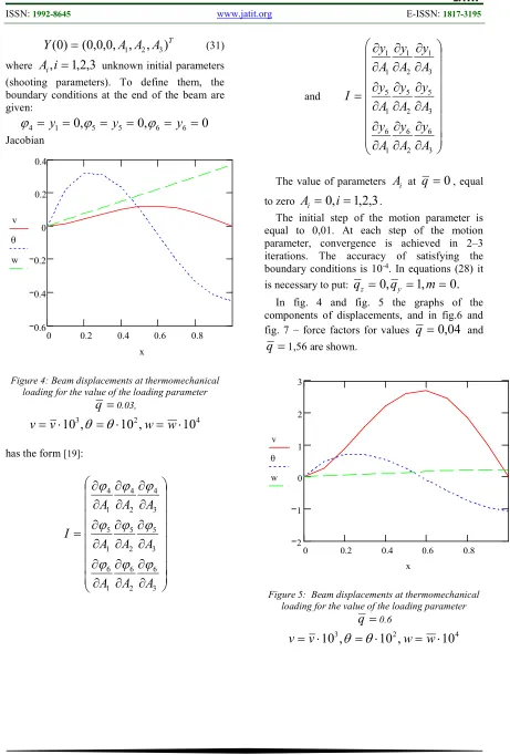
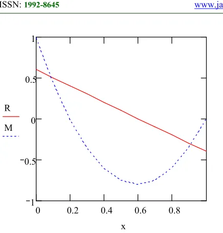
In fig. 4 and fig. 5 the graphs of the components of displacements, and in fig.6 and fig. 7 – force factors for valuesq
0
,
04
and
q
1,56 are shown.0 0.2 0.4 0.6 0.8
2 1 0 1 2 3
v
w
x
Figure 5: Beam displacements at thermomechanical loading for the value of the loading parameter
q
0.64 2
3
,
10
,
10
10
v
w
w
[image:11.612.328.547.406.580.2]4199
0 0.2 0.4 0.6 0.8 1
0.5 0 0.5 1
R M
x
0 0.2 0.4 0.6 0.8 1
0.5 0 0.5
1 1.5
R
M
[image:12.612.91.309.74.302.2]x
Figure 6: Bending moment and vertical distribution of force component under thermomechanical loading
[image:12.612.315.515.90.303.2]q
0.03R
R
,
M
M
10
Figure 7: Bending moment and vertical distribution for the value of the loading parameter
q
0.6R
R
,
M
M
10
of force component under thermomechanical loading
Comparative analysis shows that with increasing of parameter
q
the ratio between displacements changes significantlyv
andw
.5.CONCLUSIONS
1. A theoretical and computer study of the displacements, internal force factors and the temperature field during plane deformation of rods has been performed.
2. The temperature problem for a bar of rectangular cross section was studied. The differential equation of one-dimensional unsteady heat conduction is solved in the Mathcad system for boundary conditions of the first and third kind, including for non-stationary boundary conditions established experimentally. The results of numerical calculations are in good agreement with the results of the experiment and third kind, including for non-stationary boundary conditions established experimentally. The maximum error is 17% at the end of heating at
t
=440 с.3. The two-dimensional unsteady heat conduction problem is considered, when a heating device acts on a part of the rod surface. The boundary conditions on this part are written using the Heaviside function. The solution of a differential equation in partial derivatives is
carried out by the method of lines using a rectangular division grid in the Mathcad system. The generalized moments of inertia are calculated for structural carbon steels and various alloys. It has been established that the calculation of generalized geometric characteristics is essential for aluminum, magnesium and other alloys which elastic modulus changes to 24% when heated to 250– 300 0С, for structural carbon steels the elastic
modulus when heated to 250 0С changes slightly
and geometric characteristics should be used. The necessity for conducting simulation experiments in the Mathcad system will allow, in our opinion, to significantly reduce the work involved in studying the factors that affect the internal stresses and temperature fields during plane deformation of rods.
REFERENCES:
[1] Shkodkin, A., Kashirin, A., Klyuev, O., & Buzdygar, T. (2006). Metal particle deposition stimulation by surface abrasive treatment in gas dynamic spraying. Journal of Thermal Spray Technology, 15(3), pp. 382–386.
4200 development and validation of directed energy deposition additive manufacturing of Ti–6Al–4V. Additive manufacturing, 5, pp. 9–19.
[3] Bagsik, A., Schöppner, V., & Klemp, E. (2010, September). FDM part quality manufactured with Ultem* 9085. In 14th international scientific conference on polymeric materials (Vol. 15, pp. 307–315). [4] H. Assadi, F. Gartner, T. Stoltenhoff, and H.
Kreye, Bonding Mechanism in Cold Gas Spraying, Acta Mater., 2003 51(15), pp. 4379–4394.
[5] A.P. Alkhimov, V.F. Kosarev, and A.N. Papyrin, The Method of Cold Gas Dynamic Spray, Dokl. Akad. Nauk SSSR, 1990, 315(5), pp. 1062–1065.
[6] C.F. Rocheville, “Device for Treating the Surface of a Workpiece,” U.S. Patent 3,100,724, Aug 13, 1963.
[7] A. Papyrin, Cold Spray Technology, Adv. Mater. Process 2001, 159(9), pp. 49–51. [8] R.C. Dykhuizen, M.F. Smith, D.L. Gilmore,
R.A. Neiser, X. Jiang, and S.J. Sampath, Impact of High Velocity Cold Spray Particles, J. Therm. Spray Technol., 1999, 8(4), pp. 559–568.
[9] H. Assadi, F. Gartner, T. Stoltenhoff, and H. Kreye, Application of Analytical Methods for Understanding and Optimization of Cold Spray Process, Proc. Sixth Colloquium on HVOF Spraying, Nov 27–28, 2003 (Erding, Germany), pp. 49–59.
[10]O.F. Klyuev, A.I. Kashirin, T.V. Buzdygar, and A.V. Shkodkin, Equipment “DYMET” for Applying of Metal Coatings at the Manufacturing and Repair of Machine Parts, Svarochnoe Proizvodstvo, 2005, 9, pp. 43– 47.
[11]A.N. Papyrin, S.V. Klinkov, and V.F. Kosarev, Modeling of Particle-Substrate Adhesive Interaction Under Cold Spray Process Cold Spray 2004: An Emerging Spray Coating Technology, Sept 27–28, 2004 (Akron, OH), ASM International, 2004.
[12]T.V. Buzdygar, A.I. Kashirin, O.F. Klyuev, and Yu.I. Portnyagin, “Method for Applying Coatings,” Russian Federation Patent 2,038,411. June 27, 1993.
[13]A.I. Kashirin, O.F. Klyuev, and T.V. Buzdygar, “Apparatus for Gas-Dynamic Coating,” U.S. Patent 6,402,050, June 11, 2002.
[14]Kikvidze O.G., Baysarova G.G. Eksperimentalnoe issledovanie peremeshcheniy i temperaturnogo polya v sterzhne pri termomekhanicheskom nagruzhenii // Georgian engineering news, No. 3, 2015, pp. 41–44.
[15]Kikvidze O.G., Baysarova G.G. Ustoychivost sterzhnya pri neravnomernom termomekhanicheskom nagruzhenii // Georgian engineering news, No.1, 2016, pp. 45–51.
[16] Baisarova G., Kikvidze O. Experimental investigation of beam at thermo mechanical loading // VI Annual meeting of the Georgian mechanical union 30.09-4.10.2015 Tbilisi, Georgia.
[17]Kikvidze O., Baisarova G. Non stationary problem of beam’s deformation at thermo mechanical loading//Kutaisi. Bulletin of Akaki tsereteli state university №2(4), 2014, pp. 77–82.
[18]Tikhonov, U., etc. Development of on Tological Approach in E-learning When Studying Information Technologies, Eastern-European Journal of Enterprise Technologies, Vol. 5, Iss. 2, 2016, pp. 13– 20.
[19]Tvalchrelidze A., Baisarova G. Some Applications of the Theory of Shells with the Use of Several Basic Surfaces., Kutaisi, Georgia
[20]Akhmetov, B., Lakhno, V., & Oralbekova, A. Methods and Models of Self-Trained Automated Systems Detecting the State of High-Speed Railway Transport Nodes. Journal of Theoretical and Applied Information Technology, 2019, 97(9), pp. 2466–2479.
[21]Pikus, G. A., & Brzhanov, R. T. (2018, November). Assessment of concrete strength development in winter. In IOP Conference Series: Materials Science and Engineering (Vol. 451, No. 1, p. 012075). IOP Publishing.
[22]Khilenko, V.V., Strzelecki, R., Kotuliak, I., Solving the Problem of Dynamic Adaptability of Artificial Intelligence Systems that Control Dynamic Technical Objects, Cybernetics and Systems Analysis, Vol. 54, Iss. 6, 2018, pp. 867–873.
4201 [24]Lakhno, V., Kasatkin, D., Buriachok, V.,