5048
CLASSIFICATION AT INCOMPLETE TRAINING
INFORMATION: USAGE OF GROUP CLUSTERING TO
IMPROVE PERFORMANCE
1,2VLADIMIR BERIKOV, 3YEDILKHAN AMIRGALIYEV, 4LYAILYA CHERIKBAYEVA, 5DIDAR YEDILKHAN, 6BAKYT TULEGENOVA
1 Sobolev Institute of Mathematics, Novosibirsk, Russia
2Novosibirsk State University, Novosibirsk, Russia
3Suleyman Demirel University, Kazakhstan
4Institute of Information and Computational Technologies CS MES RK, Kazakhstan
5Al-Farabi Kazakh National University, Kazakhstan
6Kazakh National Research Technical University after K. Satpayev, Kazakhstan
E-mail: 1[email protected], 2[email protected], [email protected], 3[email protected] 4yedilkhan@gmail., 5[email protected]
ABSTRACT
In this paper, we propose a method for semi-supervised classification based on a group solution to cluster analysis in combination with Laplacian regularization of similarity graph. The averaged co-association matrix obtained with the cluster ensemble is considered as a similarity matrix in the regularization context. We use a low-rank representation of the matrix that allows us to speed-up computations and save memory in the solution of the derived system of linear equations. Both theoretical studies and numerical experiments on artificial data and hyperspectral imagery confirm the efficiency of the method.
Keywords: Co-Association Matrix, Cluster Ensemble, Low-Rank Representation, Semi-Supervised Learning.
1. INTRODUCTION
In pattern recognition problems, an ultimate goal is to perform a classification of sample objects described with a given feature set. With that, it is necessary to obtain an optimal value of a certain quality criterion (for example, to minimize the estimated error probability). A classifier is found using a training sample consisting of precedents – the objects with known classes they belong to. In the basic variant of the problem, class labels are known for all sample objects (fully supervised classification).
In the given work we consider another variant – the task of semi-supervised classification. In this problem, class labels are known only for a part of the given sample; it is necessary to classify either available unlabeled objects or formulate a decision rule for new objects attributing to classes. This task is urgent due to the following reasons: as a rule, unlabeled data “are cheap” (in the case when the identification of classes is an expensive procedure); usage of unlabeled data jointly with
labeled samples often allows one to involve additional information and provide significant improvement of the classification quality.
Problems of such type arise in many applied areas, for example, in the analysis of tomographic images, when a specialist indicates the belonging of some image area to one or another class (tumor, degenerative changes, etc.). Manual segmentation of the images is rather time-consuming; often only a small part of available images, therefore, can be annotated.
5049 dimensions correspond to spatial coordinates, and the third one corresponds to a spectral coordinate; therefore a hyperspectral image is called a spatial-spectral cube [3]. In many cases, the attributing of pixels to classes (vegetation or urban area types, etc.) requires field research and labeling for that reason is incomplete.
There exist a large enough number of approaches and algorithms for semi-supervised classification [4]. Currently, there are widely used self-training heuristic algorithms, probabilistic methods, transduction support vector machine (TSVM), as well as the theoretic-graph approach (Graph Laplacian Regularization) [5-8]. This approach (known also as manifold regularization) assumes that if two data points belong to the same manifold, then with a large probability they share their class labels. Laplacian graph is used for measuring the smoothness degree in the manifold including both labeled and unlabeled data. To get an efficient solution, a combination of supervised
and unsupervised classification (clustering) is
acknowledged in the literature [9].
In cluster analysis, a group (ensemble) approach is actively developing [10-11]. The application of this approach allows one to reduce the dependence of grouping results on the choice of algorithm parameters and to obtain more stable solutions in the conditions of noisy data. The idea of constructing group solutions based on the composition of simple algorithms is actively used in modern theory and practice of machine learning and data mining. A collective decision function combines the advantages of each of the methods used in constructing a classifier. Besides that, the area of its best “competence” can be determined for each of the basic decision functions.
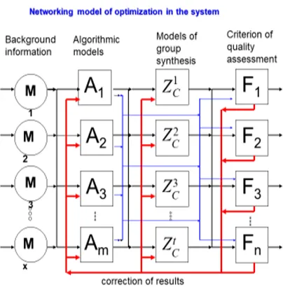
Conceptually, the optimization model of applying the group solutions (cluster ensemble) is proposed in the following scheme below. The basis of the model has been offered in [12].
In Figure 1 the points М1,М2,...,Мα denote
input data, which can be represented both as numeric values and images. A={A1, A2,…, Am} is a
set of classification algorithms, operating on different principles. 𝑧 , 𝑧 ,…, 𝑧 are algorithms of group solutions (cluster ensemble). Every 𝑧 ∊𝑧 , i 1,2,…,t makes a decision based on outcomes ofthe set of algorithms A. Further, through F={F1,
F2,…,Fn} we denote the quality criteria (validity) of
algorithms both of the first level from А, and the second level from 𝑧 . The offered model allows scaling the multitudes А and 𝑧 dimensionality. The arrows directions in the model show the data stream
subject to processing. As it is shown in Figure 1, the optimization model is presented as the networking model. One might exit from the network upon obtaining an appropriate result in terms of performance functionals.
A practical application of cluster analysis has been contemplated in the work [13]. The authors have applied a tree-like Bayesian network and k-means for computing the conventional linear Gaussians for classification of positions in motion in a dance. The basic task for using cluster analysis is recognizing a dancer’s head motions, which in turn, play a considerable role in recognizing the whole body’s gestures.
The works [14-15] offer an approach to neural network construction, which is not supported with a traditional one, based on the functional minimization. Rather, that approach is based on the operator’s theory, developed by Yu.I. Zhuravlyev [16] for solving the tasks of identification and classification.
5050 Figure 1. Concept scheme (networking model) of cluster
ensemble optimization results
The main limitations of the existing methods for semi-supervised classification are in the following:
- large computational complexity and memory demands;
- poor resistance to noise.
One of the serious problems in constructing an ensemble solution is the considerable complexity of the used search procedures. Existing algorithms are unable to analyze large-volume data.
In this paper, a computationally efficient ensemble algorithm is proposed that is able to work with a large amount of data being analyzed. This article develops a collective approach in the context of its application to the analysis of hyperspectral images. We suggest a new method of semi-supervised classification using a combination of theoretical-graph approach, regularization technique and cluster ensemble. The idea of the method is in the usage of the averaged co-association matrix as a similarity matrix in the regularization context, as well as in a low-rank presentation of the matrix to decrease the demanded memory and computation cost. The usage of group clustering aims at increasing the quality and stability of results.
In [20-21], a novel approach combining ensemble clustering and kernel-based learning was suggested for classification and regression analysis. The main idea is to consider the averaged co-association matrix calculated on the outputs of the ensemble as a similarity (kernel) matrix. Such a replacement has several grounds. Firstly, it might
be assumed that objects from the same dense region (cluster) in the feature space have common class attributes, even if the given region has a complex form. From that point of view, such points are more similar to each other, than other points which are remote from each other on the same distance but belonging to different clusters. Secondly, it is known that the averaged co-association matrix defines a semi-metric on observation space [22]; it means that the frequencies of assigning object pairs to common clusters can be considered as similarity measures for corresponding data points. The obtained matrix depends on the outputs of clustering algorithms and often is less dependent on outliers than a conventional similarity matrix.
Theoretical analysis using different kinds of ensemble models [24-25] shows that the usage of group approach allows one to raise the stability of clustering results in case of uncertainty in data structure which occurs, for instance, when the true number of clusters is unknown; or when unnecessary, noisy features are used; if data have unknown complex structures (e.g., spiral-like, spherical clusters ).
The work [26] suggests an algorithm of semi-supervised classification using a low-rank representation of the co-association matrix and linear algebraic transformations. However, in many applied tasks, these transformations are intractable due to large complexity of the problem and consequently a large size of the ensemble. In this work, we suggest the usage of efficient iterative algorithms of solving a system of linear equations instead of troublesome matrix inversion procedures. The main contribution of this paper, in comparison with other works in the field, is in the involving efficient gradient descent iterative algorithms for an approximate solution of systems of linear equations to find the predicted class labels. We also consider a new application of the developed algorithm in the problem of
hyperspectral imagery semi-supervised
classification.
The paper aims at validating the proposed methodology and summarizing our previous work. Further, in the article we give a mathematical problem statement, made a short overview of existing methods for semi-supervised classification. We describe the suggested method, discuss its properties and carry out an experimental evaluation. Finally, we give some concluding remarks.
5051
CLASSIFICATION AND RELATED WORK
Let there be an entire population 𝛤 of recognizing objects and finite set of class labels C={c1,…,ck,…,cK}. Each object 𝑎𝜖𝛤 is described
with attributes (feature set) X=(X1,…, Xd). Let us
denote through 𝑋 𝑎 the Xj attribute value for
the object 𝑎. Depending on the values and admissible operations with them, the attributes are of the following types:
- binary feature: 𝑋 𝑎 ∈ 0,1 ; - quantitative feature: 𝑋 𝑎 ∈ 𝑅; - categorical feature: 𝑋 𝑎 ∈ 𝐺: a finite set of unordered values;
- ordered feature: 𝑋 𝑎 ∈ 𝐷 : a finite ordered set.
In this work, we will consider only quantitative attributes. Under the prescribed attributes, the set 𝑥 𝑎 𝑋 𝑎 , … , 𝑋 𝑎 is called a feature description (observation) of the object 𝑎 ∈ 𝛤 . Let there be a data sample
𝑿 ={ 𝑥 , … , 𝑥 } of observations for objects
𝑎 , … , 𝑎 , where xi=x(ai). In the problem of
semi-supervised classification there are two types of samples:
𝑿𝟏 𝑥 , … , 𝑥 : describes objects
𝑎 , … , 𝑎 with known class labels 𝒀𝟏
𝑦 , … , 𝑦 , where 𝑦 ∈ 𝐶 is the label of the class to which the object ai, i=1,…,n1 belongs;
𝑿𝟎 𝑥 , … , 𝑥 is a description of
unlabeled objects (without loss of generality, we assume, that the first 𝑛 sample objects are labeled, and the next in ones are unlabeled).
There exist two main versions of the problem statement. In the first version it is demanded to conduct inductive teaching, i.e., to construct a classifier 𝑓: 𝑋 → 𝑌 which attributes class labels to objects from X0 and arbitrary new observations. In the second variant of the problem statement it is necessary to carry out transduction learning, that is to define the class labels 𝒀𝟎
𝑦 , … , 𝑦 only for the objects from X0. Both
in the first and second cases there is used some quality functional of classification. The given work considers the second version of the problem statement.
Let us consider some most frequently used approaches to supervised learning.
2.1. Self-training
In this approach, there is used some basis fully supervised classification algorithm. At the first step, the algorithm is trained at the labeled sample and
further classifies the unlabeled part. For each classified object there is computed a recognition quality estimate (for instance, the distance to the separating hyperplane). At the next step, those observations for which the quality estimate is higher than the prescribed threshold, are excluded from X0 and added to X1, and their labels replenish the set Y1. Subsequently, the basic algorithm is applied again to training on the integrated sample and classification of the remained unlabeled part. The procedure is repeated until no unlabeled objects remain.
The methods based on this heuristic procedure, as a rule, are enough effective, however theoretical analysis of their properties is a troublesome problem.
2.2. Probabilistic approach
For the given approach, it is assumed that for each class there exists a conditional distribution pj(x|𝜃 ) in feature space, where 𝜃 is a set of
distribution parameters, k=1,…,K. It is supposed the distribution type is known (for instance, normal), and its parameters should be evaluated by sample. Let us denote 𝜃 𝜃 , … , 𝜃 , and let 𝑞 𝑞 , … , 𝑞 be a set of classes prior probabilities. Then for the labeled point 𝑥 𝜖𝑿𝟏, for which yi=ck,
according to the chain rule, we obtain: p(xi,yi |𝜃 𝑞 𝑝 𝑥 | 𝜃 )
According to total probability formula, for unlabeled point 𝑥 ∈ 𝑿
p(xi |𝜃 ∑ 𝑞 𝑝 𝑥 | 𝜃 .
It is possible to consider the problem of likelihood maximization:
𝑞∗, 𝜃∗ =arg max
, ∑ log 𝑝 𝑥 , 𝑦 |𝜃
∑ log 𝑝 𝑥 |𝜃
s.t.: ∑ 𝑞 1, ∀𝑖, 𝑞 0.
The solution can be found by iterative algorithms, for example, EM algorithm for distribution mixtures [27]. After specifying the optimal 𝑞∗
𝑞∗, … , 𝑞∗ , 𝜃∗ 𝜃∗, … , 𝜃∗ , the classification of the unlabeled objects is performed according to
k
5052 Bayes formula:
𝑓 𝑥 𝑐 ∗,
where
𝑘∗ 𝑎𝑟𝑔 𝑚𝑎𝑥 𝑞∗𝑝 𝑥 |𝜃∗ , i=n
1+1,…,n
A disadvantage of the approach is in the fact that upon the significant violation of the assumptions on the probabilistic model, the found decisions have poor accuracy.
2.3. Transduction support vector machine
The basis of the given method is Support Vector
Machine (SVM) methodology for binary
classification (which can be extended to a multiclass problem). In the basic statement, it is needed to find the hyperplane for which the separating margin width is maximal. The input is a training sample X with class labels Y={y1,…,y1},
𝑦 ∈ 1, 1 , i=1,…,n. In the case of linear
separability, there exists an infinite number of separating hyperplanes. It is reasonable to select the hyperplane, the distance from which to both classes is maximal. The points lying at the margin border are called support vectors.
Let us present the hyperplane equation in the form 〈𝑤, 𝑥〉 𝑏 0, where 〈 , 〉 is a scalar product, w is a vector perpendicular to the separating hyperplane and b is a parameter. SVM constructs a decision function in the following form
f(x)=sign(∑ 𝛼 𝑦 〈𝑥 , 𝑥〉 𝑏
where 𝛼 ,…,𝛼 0 are some parameters; at that, the normalization condition 〈𝑤, 𝑥 〉 𝑏 1 for support vectors should be fulfilled. It is important to note that the summation is carried out only for those support vectors for which 𝛼 0.
For the transductive SVM, the hyperplane shall be drawn in the way it separates with a maximum margin width not only labeled points X1,
but also unlabeled points X0. Consequently, the
hyperplane should pass through the area with the lowest density. The optimization task can be formulated as follows:
find
Y0, w, b, ξ : ‖𝑤‖ 𝐶 ∑ 𝜉 → 𝑚𝑖𝑛
, , , ,
s.t.:
𝑦 〈𝑤, 𝑥 〉 𝑏 1 𝜉 , 𝑖 1, … , 𝑛,
ξi 0, i=1,…,n
where ξ1,…, ξn are variables which have the
meaning of the penalty value for the margin border violation, 𝐶 0 is a prescribed parameter. Consequently, there is maximized the margin width (one may show that the condition herein is equivalent to minimization of ‖𝑤‖ ), and the total penalty for the margin borders violation is minimized.
There exist algorithms for the given task approximate solution [28]; for this purpose, there is solved a corresponding dual problem for parameters α1,…,αn.
Upon a linear inseparability of classes, the transformation φ: X→X’ of the initial space X into a
new space X’ of higher dimensionality can be
performed. In the new space, the objects can already be linearly separable. A decision function f(x) depends on the vector scalar product, not on the objects immediately. Therefore the scalar product
〈𝑥, 𝑧〉 can be replaced with the products of the type
〈𝜑 𝑥 , 𝜑 𝑧 〉 in the rectifying space X’. In this case,
the decision function has the form:
f(x)=sign(∑ 𝛼 𝑦 〈𝜑 𝑥 , 𝜑 𝑥 〉 𝑏
Function K(x,z)=〈𝜑 𝑥 , 𝜑 𝑧 〉 is called a kernel. The transition from a scalar product to a kernel is a “kernel trick”.
The selection of a kernel defines an implicit transformation to rectifying space and allows applying linear algorithms (in particular, SVM) to linearly inseparable sample. For kernel-based methods, the Mercer’s theorem [29] is widely known. It establishes necessary and sufficient conditions for a function to be a kernel. According to the theorem, continuous (or defined on a finite set) function K(x,z) is a kernel then and only then, when it is symmetric: K(x,z)=K(z,x) and positive semi-definite: for any finite sample (x1,…
xp), given matrix K=(K(xi,xj)) and any 𝑧 ∈ R , it
holds true: zTKz 0.
5053 for transductive SVM is nonconvex, and known algorithms of its approximate solution are of polynomial cost. Therefore the approach can be applied to samples of comparatively small size (about a thousand observations).
2.4. Graph Laplacian regularization
Let us consider a weighted non-directed complete graph G=(V,E), in which the set of vertices V corresponds to observations from X, and the set of edges E corresponds to pairs (xi,xj), i, j=1,…,n, i 𝑗.
Each edge (xi,xj) is associated with a nonnegative
number (weight) Wij, having the meaning of the
given pair degree of similarity. For example, the weight can be defined using RBF function:
Wij=exp
where 𝜎 is a prescribed parameter.
Let 𝑌 𝑌 , … , 𝑌 denote a Boolean
vector of the observed associations with classes: 𝑌 𝑰[yi=ck], where 𝐈[ꞏ] is a predicate
function: I[true]=1, I[false]=0, i=1,…,n1, k=1,…,K.
Let us denote through Fi=(Fi1,…,FiK) a
classification vector, in which the element Fi 0
has a sense of the degree of belonging of point xi to
class cj, and let the classification matrix of
dimensionality n 𝐾 be specified as F 𝐹 , … , 𝐹 .
Let us consider the following optimization task: find
𝐹∗ arg min
∈ 𝑄 𝐹 ∑ ∈ ‖𝐹 𝑌 ‖
𝛽 ∑ 𝑿𝑊 , (1)
providing 𝐹 0, where 𝛽 0 is a regularization parameter. The first sum in the right part of (1) is aimed at minimizing the labeled data fitting error; the second component plays the role of a smoothing function: its minimization means that if two points
𝑥, 𝑥 (labeled or unlabeled) are similar, then their classification vectors shall not differ much. It is known that the function being optimized is convex. Let us introduce a diagonal matrix 𝐷 with components 𝐷 ∑ 𝑊 . The matrix
𝐿 𝐼 𝐷 / 𝑊𝐷 /
is called the normalized Laplacian, I is an identity matrix. The matrix has dimensionality 𝑛 𝑛; its
element 𝐿 equals 𝐿 𝛿 , where
𝛿 𝑰[i=j] is the Kronecker symbol. Note that there
are other variants of graph Laplacian definition [3]. To find the optimal solution, we differentiate (1), and after simple transformations obtain:
| ∗ 𝐹∗ 𝑌 +𝛽𝐹∗ 𝐿,∙𝐹∙,∗ 0 (2)
𝑖 1, … , 𝑛 ,
| ∗ 𝛽𝐹∗ 𝛽𝐿,∙𝐹∙,∗ 0, (3)
𝑖 𝑛 1, … , 𝑛
where 𝐿,∙, 𝐹∙,∗ is the ith row of matrix L and kth column of matrix 𝐹∗ accordingly, i=1,…,n
1, k=1,…,K. Let us denote through 𝑌, the matrix
𝑌, 𝑌 , … , 𝑌 , 0, … ,0
of dimensionality 𝑛 𝐾, and through 𝐼, the diagonal n 𝑛 matrix:
𝐼, 𝑑𝑖𝑎𝑔 𝐼 … , 𝐼 , 𝐼 0, 𝑖1, 𝑖𝑛1, … , 𝑛1, … , 𝑛. (4)
Then (2) and (3) can be rewritten in matrix form:
(𝐼, 𝛽𝐿)𝐹∗ 𝑌, , (5)
from which
𝐹∗ 𝐼
, 𝛽𝐿 𝑌, , (6)
if the inverse matrix exists (note that the regularization parameter 𝛽 can be chosen in the way to ensure well conditioning of the obtained task).
To find the solution, one may use iterative methods. For example, the work [6] describes Label Spreading iterative algorithm used for solving the task analogous to (6). Apart from that, we may apply existing methods for solving linear equations systems, where each system is considered concerning corresponding columns 𝐹∗, 𝑌
5054 defined according to the formula:
𝑦 𝑐 ∗
where
𝑘∗ 𝑎𝑟𝑔 max
,…, 𝐹 , 𝑖 𝑛 1, … , 𝑛. (7)
A limitation of the given approach is that it operates with non-sparse graph Laplacian matrix of dimensionality 𝑛 𝑛 which results in a large cost of matrix operations and memory demand.
3. SUGGESTED METHOD
The method is based on a combination of collective cluster analysis and theoretical graph approach. The main idea is in the usage of the averaged co-association matrix of cluster ensemble as a similarity matrix in (1).
3.1. Cluster ensemble and averaged co-association matrix
According to group approach in clustering, we consider several different clustering partitions of the same data and integrate them to find the overall consensus partition.
As a rule, each partition variant is formed according to the parameters of the clustering algorithm selected at random from an admissible set of parameters. One can also vary the algorithm’s settings (such as distance type, initialization, feature subspace) to get different variants of partitioning.
In our task, we do not need to partition data: our primary goal is to perform a classification of the unlabeled sample. The used information obtained by multiple clustering can be presented in the form of the averaged co-association matrix.
Let us consider r partition variants 𝑃 , where 𝑃 𝐶, , … , 𝐶, , 𝐶, ⊂ 𝑿, 𝐶, ∩
𝐶, =∅, 𝐾 is the number of clusters in the partition variant. For each 𝑃 we define matrix
𝐻= 𝐻 𝑖, 𝑗 , , the elements of which indicate
wether a pair 𝑥, 𝑥 belongs to the same cluster in the l-variant or not:
𝐻 𝑖, 𝑗 𝑰 c 𝑥 c𝒍 𝑥 ,
where 𝑐 𝑥 denotes the cluster label assigned to point x. Weighted averaged coassociation matrix is defined as follows:
𝐻 𝐻 𝑖, 𝑗 , , 𝐻 𝑖, 𝑗 𝑤 𝐻 𝑖, 𝑗
where 𝑤 ,…,𝑤 are weights, 𝑤 0, ∑ 𝑤 1. The weights can be identical or can be selected proportionally to some quality index of each clustering variant.
It was shown in [11] that matrix H is symmetric and positive semi-definite. Thus, according to Mercer’s condition, it is possible to use it as a kernel matrix in kernel-based classification methods such as SVM or kNN. Below we describe basic steps of algorithms CASVM and CANN which implement the combination scheme. Algorithm CASVM
Input: data set 𝑿𝟏 with known class labels 𝒀𝟏; unlabeled data 𝑿𝟎; number of clustering variants r;
Output: predicted class labels 𝒀𝟎.
Steps:
1. Generate r variants of the partition of 𝑿 𝑿𝟏∪ 𝑿𝟎 using a given clustering algorithm with randomly chosen parameters; calculate quality indices and weights 𝑤 ,…,𝑤;
2. Calculate the averaged co-association matrix Н. 3. Train SVM at labeled data 𝑿𝟏 using matrix Н as a kernel matrix.
4. Predict 𝒀𝟎 using the trained SVM.
end
Algorithm CANN:
Input: data set 𝑿𝟏 with known class labels 𝒀𝟏; unlabeled data 𝑿𝟎; number of clustering variants r;
Output: predicted class labels 𝒀𝟎.
Steps:
1. Generate r variants of the partition of 𝑿 𝑿𝟏∪ 𝑿𝟎 using a given clustering algorithm with randomly chosen parameters; calculate quality indices and weights 𝑤 ,…,𝑤;
2. Calculate the averaged co-association matrix Н. 3. Apply nearest neighbor method: for each unlabelled object 𝑥 ∈ 𝑿𝟎find a class label of the most similar (according to H) labeled object 𝑥 ∈ 𝑿𝟏:
𝑥′ 𝑎𝑟𝑔 𝑚𝑎𝑥
,…, 𝐻 𝑥 , 𝑥 .
end
5055 It was proved in [25] that under some natural assumptions on the probabilistic properties of the ensemble, the probability error in classifying an arbitrary pair of points to clusters approaches zero at increasing the ensemble size.
3.2. Low-rank representation of averaged co-association matrix
By the definition, the averaged co-association matrix requires quadratic memory with respect to sample size. Nevertheless, this requirement can be relaxed using the matrix low-rank representation.
The next property allows one to sufficiently decrease the computation cost.
Proposition. Weighted averaged co-association matrix admits low-rank representation in the form:
𝐻 𝐵𝐵 , 𝐵 𝐵 𝐵 … 𝐵 (8)
where B is a block matrix, B w A ; A is an
association matrix for lth clustering partition which has a dimensionality 𝑛 𝐾: A 𝑖, 𝑘 𝐈 c x 𝑘 , i=1,…,n, k =1,…,𝐾.
As a rule, 𝑚 ∑ 𝐾 ≪ 𝑛 ; thus (8) gives us a possibility to save memory by storing sparse matrix B of dimensionality 𝑛 𝑚 instead of full matrix H. The cost of matrix multiplication 𝐻 ∙ 𝑥 is reduced from 𝑂 𝑛 to 𝑂 𝑛𝑚 .
3.3. Cluster ensemble and graph Laplacian regularization
We consider matrix H as a similarity matrix W in (1) and define the normalized Laplacian of the corresponding graph in the form: 𝐿 𝐼
𝐷 / 𝐻𝐷 / , where 𝐷 𝑑𝑖𝑎𝑔 𝐷 , … , 𝐷 ,
𝐷 ∑ 𝐻 𝑖, 𝑗 . We obtain:
𝐷 =∑ ∑ 𝑤 ∑ 𝐴 𝑖, 𝑘 𝐴 𝑗, 𝑘
∑ 𝑤 ∑ 𝐴(j,k)= ∑ 𝑤 𝑛 𝑖 (9)
where 𝑛 𝑖 is the size of the cluster which includes the point 𝑥 in l-variant of partitioning. Substituting 𝐿 in (5), we obtain a linear equations system:
𝐼, 𝛽𝐿 𝐹∗∗ 𝑌, . (10)
Using (8), the system can be transformed
into a form that uses more effective operations with low-rank matrices. For that purpose, let us denote
𝑈 𝐷 / 𝐵, then 𝐿 𝐼 𝑈𝑈 . From (6) and (8) we obtain the system:
𝐼, 𝛽𝐼 𝑈𝑈 𝐹∗∗ 𝑌, . (11)
For the numerical solution, one can use any of the existing iterative algorithms. In the given work we use algorithm GDSolve [30] based on gradient descent. The GDSolve algorithm convergence for symmetrical positive definite system matrix was proved in [30]. Let us describe the main steps of the given GDSolveLR algorithm modification, which uses low-rank graph Laplacian representation.
GDSolveLR algorithm:
Input:
𝑈, 𝐼, : sparse matrices in the left part of (11);
𝑌, : matrix in the right part of (11);
𝛿 0: required accuracy parameter.
Output:
𝐹∗∗: classification matrix.
Steps:
1. t:=0; 𝐹∗∗ 0 ≔ 0; 2. for k:=1 → K do
3. b:= 𝑌, ∙ (kth column of matrix 𝑌, ); 4. repeat
5. compute residual error 𝑟 𝑡 ≔ 𝑏 𝐼, ∙
𝐹∙,∗∗ 𝑡 𝛽𝐹∙,∗∗ 𝛽𝑈 𝑈 ∙ 𝐹∙,∗∗ 𝑡 ; 6. find the optimal step length
𝜂 𝑡 ≔
, ∙ ∙ ;
7. 𝐹∙,∗∗ 𝑡 1 ≔ 𝐹∙,∗∗ 𝑡 𝜂(t)∙ 𝑟 𝑡 ; 8. until r(t) 𝛿;
9. endfor
10. return 𝐹∗∗ 𝑡 1 .
Note that at the steps 5,6 the algorithm performs a multiplication by Laplacian matrix represented in a low-rank form; thus it is not required to save in the memory full matrix of 𝑛 𝑛
size. Below we describe the main steps of the
proposed algorithm SSC-LR-GD for
semi-supervised classification based on Laplacian similarity graph, low-rank representation of co-association matrix and gradient method. Algorithm SSC-LR-GD:
Input:
5056 data 𝑿𝟎; number of clustering variants r;
Output:
predicted class labels 𝒀𝟎.
Steps
1. Generate r variants of the partition of 𝑿 𝑿𝟏∪ 𝑿𝟎 using a given clustering algorithm with randomly chosen parameters; calculate quality indices and weights 𝑤 ,…,𝑤 ;
2. Calculate normalized graph Laplacian in a
low-rank representation, using matrices B in (6),
𝐷 in (9) and 𝐼, in (4).
3. Find classification matrix 𝐹∗∗ with GDSolveLR algorithm;
4. Define labels for Y0, using matrix 𝐹 𝐹∗∗ in (7).
end.
In the computer implementation, we use k-means as a base clustering algorithm.
4. EXPERIMENTAL STUDY
The suggested algorithm SSC-LR-GD was evaluated in numerical experiments. The first experiment employs Monte Carlo simulation to estimate the accuracy and time complexity of the algorithm under various sample size and noise levels for a given example of data distribution. The second experiment demonstrates the applicability of the method in the real task of hyperspectral image analysis.
4.1. Mixture of normal distributions
In this example we consider data sets generated from the mixture of five multidimensional normal distributions N(ai,𝜎XI) at equal weights; 𝑎 ∈ 𝑹 , i=1,…,5, d=8; value 𝜎 is a parameter. To study the algorithm robustness under noise conditions,
two independent random features are additionally generated according to the uniform distribution
𝑈 0, 𝜎 where noise parameter 𝜎 5. Figure 2
illustrates the generated data. In the simulation process, we repeatedly generate samples of size n with the given distribution.
10% of points selected at random from each component compose a labeled part of the sample; the remaining points are included in an unlabeled subsample. Cluster ensemble variants are generated using random initialization of centroids in k-means (number of clusters equals 10). The number of ensemble elements r=10. The weights of ensemble variants are identical: 𝑤 ≡ 1 𝑟. Regularization parameter 𝛽 is evaluated by cross-validation and grid search in the interval [0.001,0.5] with a step 0.005; the best prediction has been obtained for
𝛽=0.1. Parameter 𝛿=10 .
We also apply an algorithm (denoted SSC-RBF) which uses a standard similarity matrix found with RBF kernel (parameter 𝜎 4), in which the predictions are calculated according to (6). To raise the reliability of the comparison, quality estimates (frequency of correct predictions on test sample) are averaged over 40 experiments. Analysis of the statistical significance of the differences between the estimates is performed using a paired two-sampleStudent's t-test.
Table 1 presents the results of the experiments. The table shows the averaged accuracy estimates, as well as the averaged operation time (on the dual-core Intel Core i5 processor with a clock frequency 2,8 GHz and 4 Gb RAM). For SSC-LR-GD, we separately indicate ensemble generation time and matrix operation time (in seconds). Accuracy evaluations that are statistically significantly better than those of the compared algorithm (p-value 10 ) are in bold.
Table 1. Results of experiments with distribution mixture for various sample size n and parameter 𝜎 values.
The results demonstrate that SSC-LR-GD shows comparable or even higher accuracy than SSC-RBF. For large data size (n=105, n=106),
SSC-RBF failed due to unacceptable memory demands (74.5 Gb and 7450.6 Gb correspondingly).
One can see that SSC-LR-GD spend the most time in the stage of iterative computations. The average operation time for SSC-LR-GD is much less than that for SSC-RBF which does not
SSC-LR-GD SSC-RBF
accura
cy (sec) (sec) accura
cy time (sec)
1000
1 1.000 0.06 0.10 1.000 0.32
3 0.985 0.07 0.02 0.982 0.32
5 0.874 0.13 0.11 0.817 0.35
3000
1 1.000 0.10 0.48 1.000 5.42
3 0.986 0.13 0.10 0.984 5.29
5 0.878 0.23 0.48 0.848 5.48
105 1 1.000 2.05 25.69 - -
106 1 1.000 49 443 - -
n X
[image:9.612.86.301.185.439.2]5057 use low-rank operations.
4.2. Analysis of hyperspectral images
For the experimental research of the developed algorithm, we use the Indian Pines hyperspectral image [30]. This scene was gathered by AVIRIS sensor over the Indian Pines test site in North-western Indiana. The image size is 145 145 pixels; each pixel is characterized by the vector of 224 spectral intensities in the 400-2500 nm range. Figure 3(a) shows the RGB-composite, and Figure 3(b) presents the ground truth map with 16 classes (different vegetation types). The image has unlabeled pixels which are not assigned to any of the classes. These pixels are excluded from the analysis.
In the experiment, the labeled part comprises 1% of points selected at random for each component. To reduce the spectral channels correlation effect, we use PCA to decrease the dimensionality up to 10 features.
The transformed data is used as input for SSC-LR-GD. Ensemble size r=10; base ensemble elements are generated with cluster number variation in the interval [1000, 1000+r]. The other parameters coincide with the described ones in the previous experiment.
[image:10.612.307.529.37.182.2]We also perform a comparison with multiclass SVM which uses standard RBF kernel (with parameters recommended by default).
Figure 2. Generated data (projection on axes X1, X2):
n=1000, 𝜎 1
Figure 3. Indian Pines hyperspectral image: (a) composite image of hyperspectral data; (b) ground-truth
map
To increase the statistical reliability of the comparison, we average the accuracy estimates over 20 runs for each algorithm with randomly selected labeled subsamples. At each run, we calculate classification accuracy estimate on the unlabeled pixels which are not used at the training stage. For SSC-LR-GD, the average operation time is about 1.5 minutes, and for SVM about 0.3 minutes. As a result, the SSC-LR-GD average accuracy is 0.657, and that of SVM 0.613. A paired Student’s t-test has shown a significant improvement in the accuracy of SSC-LR-GD (p-value < 10-5).
We also have examined CASVM
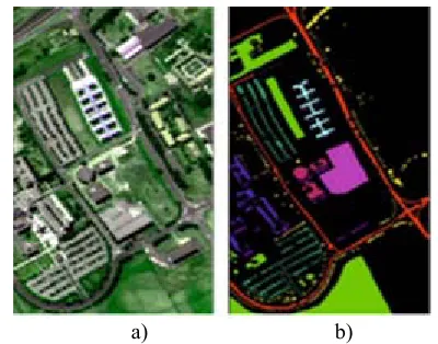
performance on another hyperspectral image. We use Pavia University scene [31], which has a size of 610 340 pixels, containing 103 spectral channels. The spatial resolution of the scene is 1.3 m. Figure 4а) shows the image’s RGB-composite (channels 40, 50 and 70), and Figure 4b) presents the ground truth map.
There are unlabeled pixels in the image which are not assigned to one of the nine classes. The given pixels are excluded from the consideration.
[image:10.612.97.286.483.690.2]a) b)
[image:10.612.316.516.532.689.2]5058 In the experimental study, 1% of the pixels selected at random for each class compose a labeled sample; the remaining ones are included in the unlabeled part. To study the effect of noise on the quality of algorithms, we add normally distributed noise to the spectral brightness values: a corresponding value x is replaced by a quantity x(1+pε), where p is a parameter, ε follows standard normal distribution.
An obtained data consisting of the spectral intensity values of the pixels over all channels is an input of CASVM. K-means is chosen as a base algorithm for constructing a cluster ensemble. Different variants of the partitioning are generated by varying the number of clusters in the interval [30,30+r] where r=120. To speed up the operation time of k-means and obtain more diverse results, the number of iterations is limited to 1.
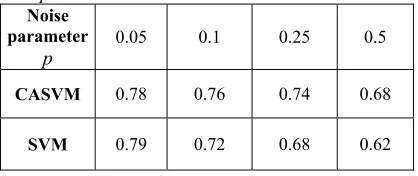
[image:11.612.91.300.372.460.2]Table 2 shows the accuracy estimates in the classification of unlabeled pixels for some pairs of noise parameters.
Table 2. Accuracy of CASVM and SVM at some values of noise parameters
Noise parameter
p 0.05 0.1 0.25 0.5
CASVM 0.78 0.76 0.74 0.68
SVM 0.79 0.72 0.68 0.62
The running time of the algorithm is about 2 minutes. As can be seen from the table, CASVM algorithm is more noise resistant than SVM.
6. CONCLUSION
In this work, we have considered a pattern recognition problem in case of incomplete training information. Using a combination of the methodologies, based on the regularization of Laplacian similarity graph, collective cluster analysis, and a low-rank matrix representation, a method for the solution of the given task was suggested.
The main idea of the method is in the usage of the averaged co-association matrix of cluster ensemble as a similarity matrix in graph Laplacian regularization context. The matrix admits a low-rank representation that has allowed us to speed-up computations and save memory in the solution of the derived system of linear equations (from quadratic to linear concerning sample size).
We have performed an experimental study of the suggested method by the usage of Monte Carlo simulations. In the experiments, the method has shown comparable or even significantly better accuracy estimates than an analogous algorithm, not using group clustering and a low-rank representation of the co-association matrix. In the case of a big volume of data (up to a million points), the standard algorithm failed due to the infeasible memory requirements, and the proposed method gave an accurate solution in a few hundred seconds running on an ordinary computer. Even for a small amount of data, the average working time of the suggested algorithm turned out to be much less than that of the analogous standard one.
In the experimental study on the real hyperspectral image in noise conditions, the suggested methodology has allowed obtaining more accurate solutions than the existing SVM technique.
Further, we plan to continue the theoretical study of the suggested method (to investigate the problem of theoretical convergence to an optimal solution in the probabilistic context, to obtain classification quality estimates). To accelerate the computations, there are good reasons to vectorize the proposed algorithm upon forming a cluster ensemble and use more effective procedures for solving a linear equations system.
ACKNOWLEDGMENTS
The work was supported by the program of Fundamental Scientific Researches of RAS, project № 0314-2019-0015 of the Sobolev Institute of mathematics. The research was partly supported by RFBR grant 19-29-01175.
REFRENCES:
[1]Bondur, V.G.Modern approaches for processing of big hyperspectral aerospace data//Earth Observation and Remote Sensing. 2014. No. 1. P. 4–16. (In Russ.)
[2]Abdiakhmetova Z.M. Wavelet Data Processing In The Problems Of Allocation In Recovery Well Logging. Journal of Theoretical and Applied Information Technology, 2017 Volume_8, P.1041-1047.
[3]Schowengerdt, R.A. Remote sensing: models and methods for image processing. New York: Acad. Press, 2006. 560 p.
5059 [5]Camps-Valls G., Marsheva T., Zhou D.
Semi-supervised graph-based hyperspectral image classification // IEEE Transactions on Geoscience and Remote Sensing. 45(10). 2007. P. 3044-3054.
[6]Wu M., Scholkopf B. Transductive
Classification via Local Learning
Regularization // Artificial Intelligence and Statistics. 2007. P. 628-635.
[7]Zhou D., Bousquet O., Lal T., Weston J., Scholkopf B. Learning with local and global consistency // In Advances in Neural Information Processing Systems. 16, 321-328. 2003.
[8]Belkin M., Niyogi P., Sindhwani V. Manifold Regularization: A Geometric Framework for Learning from Labeled and Unlabeled Examples // J. Mach. Learn. Res. Vol. 7, no. Nov. 2399-2434. 2006.
[9]Yu G. X., Feng L., Yao G. J., Wang, J. Semi-supervised classification using multiple clusterings // Pattern Recognition and Image Analysis. 26(4), 681-68. 2016.
[10] Boongoen T., Iam-On N.: Cluster ensembles: A survey of approaches with recent extensions and applications. Computer Science Review. 28, 1-25, 2018..
[11] Berikov V. Weighted ensemble of
algorithms for complex data clustering // Patt. Recogn. Lett. 2014. Vol. 38. P. 99–106.
[12] Amirgaliyev E.N., Mukhamedgaliev A.F. An optimization model of classification algorithms // USSR Computational mathematics and mathematical physics. 1985, 6, Р. 95-98. [13] Nussipbekov A.K., Amirgaliyev E., Hahn M.
Kazakh traditional dance gesture recognition. Journal of Physics: Conference Series. Vol. 495, Issue 1, 2014
[14] Dyusembaev A. E., Grishko M.V.
Construction of a Correct Algorithm and Spatial Neural Network for Recognition Problems with Binary Data. Computational Mathematics and Mathematical Physics. Vol. 58, Issue 10, p. 1673-1686, 2018
[15] Dyusembaev A., Grishko M. On Correctness Conditions for Algebra of Recognition Algorithms with Operators over Pattern Problems with Binary Data. Doklady mathematics Vol.: 98 No. 2 p. 421-424, 2018.: 236-239
[16] Zhuravlev Yu.I., Nikiforov V.V. Algorithms for recognition based on calculation of evaluations // Kibernetika. 1971. Vol. 3. P. 1– 11.
[17] Kenshimov C., Bampis L., Amirgaliyev B., Arslanov M., Gasteratos A. Deep learning features exception for cross-season visual place recognition. Pattern recognition letters. Vol. 100,p. 124-130, 2017.
[18] Merembayev T., Yunussov R., Amirgaliyev Y. Machine Learning Algorithms for Stratigraphy Classification on Uranium Deposits. Procedia Computer Science. Vol.: 150, p. 46-52, 2019. [19] Amirgaliev E., Isabaev Z., Iskakov S., Kuchin
Y., Muhamediyev R., Muhamedyeva E., Yakunin K. Recognition of rocks at uranium deposits by using a few methods of machine learning // Advances in Intelligent Systems and Computing. Vol. 273, p. 33-40, 2014.
[20] Berikov V., Karaev N., Tewari A. Semi-Supervised Classification with Cluster Ensemble // Proceedings of 2017 International Multi-Conference on Engineering, Computer and Information Sciences (SIBIRCON). Novosibirsk, Russia. 18-22 Sep 2017. P. 245-250.
[21] Berikov V., Vinogradova T. Regression analysis with cluster ensemble and kernel function // Lecture Notes in Computer Science, Vol. 11179. 2018. P. 211-220.
[22] Berikov V.B. Construction of an optimal collective decision in cluster analysis on the basis of an averaged co-association matrix and cluster validity indices // Pattern Recognition and Image Analysis. 27(2), 153-165. 2017. [23] Berikov V., Pestunov I. Ensemble clustering
based on weighted co-association matrices: Error bound and convergence properties // Pattern Recognition. 2017. Vol. 63. P. 427-436.
[24] Berikov V., Cherikbayeva L. Searching for Optimal Classifier Using a Combination of Cluster Ensemble and Kernel Method //
OPTA-SCL 2018. CEUR Workshop
Proceedings. Volume 2098, 2018, P. 45-60. [25] Amirgaliyev Y., Berikov V., Latuta K.,
Bekturgan K., Cherikbayeva L. Group Approach to Solving the Tasks of Recognition // Yugoslav Journal of Operations Research, 2019. 2, P. 177–192.
5060 [27] Dempster A.P. Laird N.M. Rubin D.B.
Maximum Likelihood from Incomplete Data via the EM Algorithm // Journal of the Royal Statistical Society, Series B. 39 (1): 1–38. 1977. [28] Collobert R. et al. Large scale transductive
SVMs // Journal of Machine Learning Research, 7, pp.1687-1712. 2006.
[29] Mercer J. Functions of positive and negative type and their connection with the theory of integral equations // Philosophical Transactions of the Royal Society A, 209. 1909. P. 415–446. [30] Vishnoi, Nisheeth K. Lx=b Laplacian Solvers
and Their Algorithmic Applications // Foundations and Trends in Theoretical Computer Science 8.1–2. 2013. P. 1-141. [31] Hyperspectral Remote Sensing Scenes. (2019,
April 17). Retrieved