Indexed Tree Sort: An Approach to Sort Huge Data with
Improved Time Complexity
Prateek Agrawal
Department of Computer Science & Engineering Lovely Professional University
India
Harjeet Kaur
Department of Computer Science & Engineering Lovely Professional University
India
Gurpreet Singh
Department of Computer Science & Engineering Lovely Professional University
India
ABSTRACT
Sorting has been found to be an integral part in many computer based systems and applications. Efficiency of sorting algorithms is a big issue to be considered. This paper presents the efficient use of Indexing with Binary Search Trees (BST) to model a new improved sorting technique, Indexed Tree (IT)-Sort, capable of working with huge data. Along with design and implementation details, major emphasis has been placed on complexity, to prove the effectiveness of new algorithm. Complexity comparison of IT-Sort with other available sorting algorithm has also been carried out to ascertain its competence in worst case also. In this paper, we describe the formatting guidelines for IJCA Journal Submission.
Keywords
Computing, Sorting Algorithm, Complexity, Huge Data Set, Binary Search Tree (BST), Indexing
1.
INTRODUCTION
There are number of traditional algorithms used to find ordering of unordered data sets. Each algorithm has its own pros and cons and a specific methodology to arrange the data like merging divide and conquer, partitioning, recursive methods etc [1, 2]. Different sorting algorithms are analyzed and compared according to their complexity [3, 6, and 7]. The analysis of algorithms is the area of computer science that provides tools for contrasting the efficiency of different methods of solution. Although the efficient use of both time and space is important, inexpensive memory has reduced the significance of space efficiency [4]. Thus, focus of researcher has been restricted to primarily on time efficiency only. Time complexity of an algorithm is a function of the size of the input to the problem and quantifies the amount of time taken by an algorithm to execute. Designing of suitable sorting algorithm as per application is a continuous process. Lots of work is being carried out in this field with single objective to reduce time complexity of proposed algorithm. Existences of large number of data values have significant impact on computational complexity of sorting. Since, sorting large datasets may slowdown the overall execution, schemes to
to a great extend if sorting is carried out with huge data sets even in worst case. In this paper, an attempt has been made to present improved approach for finding more efficient solution, requiring less execution time, of sorting using Indexing and BSTs.
The rest of the paper is organized as follows. Next section describes the methodology followed in designing IT-Sort. Main emphasis in section 3 has been placed on presenting the design and implementation details of new algorithm. Section 4 supports the whole discussion with experimental results to prove the effectiveness of proposed algorithm and finally section 5 concludes the paper with future enhancements.
2.
IT-SORT
2.1
Enhanced Algorithm for Sorting
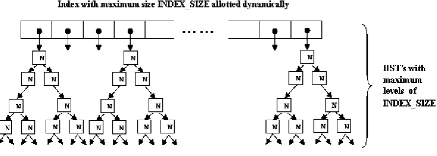
to be an array of pointers. In order to create an index of BSTs, two special kinds of structures are created. First one is to access the indexed items and another to represent the node in a BST. As shown in Figure 1(a and b), we use a pointer-based linear list structure to implement Indexed BSTs. Each node of the list contains a link to one BST with index value equal to the node number and a reference down pointer to point the next node of the list.
An array of pointers to BSTs, index_bst has been used to represent an element in Index List. Pointer arrays offer a particularly convenient method for representing these index values. An n element array can point to n different BSTs. Each individual BST can be accessed by referring to its corresponding pointer. An advantage to this scheme is that a fixed block of memory needs not to be reserved in advance, as is done when initializing a conventional array. Moreover, size of the index list varies according to values in the list to be sorted. Maximum value from the unordered list is taken to determine the size of the list. If max_value represents the biggest value in unsorted list, then size is calculated as per
following formula
INDEX_SIZE = sqrt(MAX_VALUE)
Memory is dynamically allocated to index list according to calculated array_size as
INDEX_BST = ( int * ) malloc ( INDEX_SIZE * sizeof ( int ) )
Since an array name is actually a pointer to the first element within the array, it is more convenient to define array as a pointer variable. In order to calculate the address of any element, one must specify only the array name and number of elements beyond the first. An important advantage of dynamic memory allocation is the ability to reserve as much memory as may be required during program execution and then release this memory when it is no longer needed.
Figure 1(a): Pointer based dynamic linear list structure for Indexed BST
[image:2.595.76.522.304.463.2]Apart from array_bst, one another significant structure is BST_Node defined as
typedef struct BST_Node {
BST_Node*l_node; int data;
BST_ node*r_node; }
Each node of binary search tree will contain l_node to point to left BST, r_node to point to right BST and an integer data to hold value. In order to deal with duplicate values in data set, a separate counter has been associated with each data item. The major advantage of using binary search trees over other data structures is that the related traversal is very efficient. An in order tree walk will produce arranged data in sorted order.
3.
DESIGN OF PROPOSED
TECHNIQUE
3.1 Efficient Solution
The algorithm for IT Sort is presented below in Figure 2. The complete algorithm has been divided into two different modules. Before the application of IT Sort, data items are required to be placed in appropriate locations. Second module CREATE_INDEX() is responsible for making the indexed tree of data items. This function creates indexed tree of a list LIST with N items and returns starting address of the index INDEX_BST and size of the index INDEX_SIZE. INDEX_BST is a pointer indicating the start of the index with INDEX_SIZE entries. Value of N is supposed to be very large. Function FIND_MAX() calculates the largest value in the LIST, MAX_VALUE and later on this MAX_VALUE is utilized in calculating the size of the index INDEX_SIZE. Once the size is known, function malloc() dynamically allocates INDEX_SIZE blocks of memory for index in IT Sort. The starting address of the allocation is assigned to INDEX_BST. Step 4 in the algorithm arranges the data items in LIST in a binary search tree at corresponding index entry. LIST is read till the end, for every read data item LIST_ITEM, CALCULATE_INDEX_POINTER() is called to find its relevant index pointer. The address returned by this function, ROOT serve as root address of its corresponding BST. INSERT_BST() adds the LIST_ITEM in a BST at ROOT after finding its appropriate placement in BST. Function IT_SORT() includes two basic steps of creating indexed tree and in order reading of BSTs. In first step function CREATE_INDEX is called which returns the beginning of the indexes INDEX_BST and number of indexes to be processed INDEX_SIZE. For every index starting from INDEX_BST to INDEX_SIZE, in order traversal of binary search tree INORDER() is made. A simple iterative loop has been applied to in order traverse the different binary search
IT_SORT ( LIST , N )
// This algorithm sorts LIST with N items.
Step 1: CREATE_INDEX ( LIST , N , INDEX_BST , INDEX_SIZE )
Step 2: Repeat for I = 1 to INDEX_SIZE
a) Print INORDER ( INDEX_BST)
b) INDEX_BST = INDEX_BST + 1
Step 3: Exit
CREATE_INDEX (LIST , N , INDEX_BST ,
INDEX_SIZE )
// This algorithm creates index tree of LIST with N items and returns the starting address of index INDEX_BST and size of index INDEX_SIZE
Step 1 : MAX_VALUE = FIND_MAX ( LIST )
Step 2 : INDEX_SIZE = sqrt ( MAX_VALUE )
Step 3 : INDEX_BST = malloc ( INDEX_SIZE )
Step 4 : While Not ( End of LIST ) Repeat
(a) Read LIST_ITEM
(b) ROOT = CALCULATE_INDEX_POINTER (
LIST _ITEM )
(c) INSERT_BST (LIST_ITEM , ROOT )
Step 5 : Exit
Figure 2: Psuedocode for IT_SORT
3.2 Implementation Details
4.
TESTS AND RESULTS
4.1 Examples
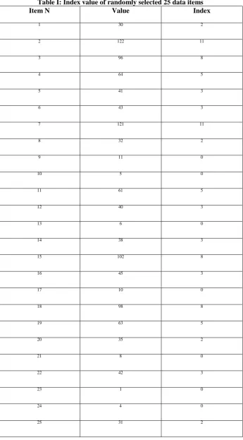
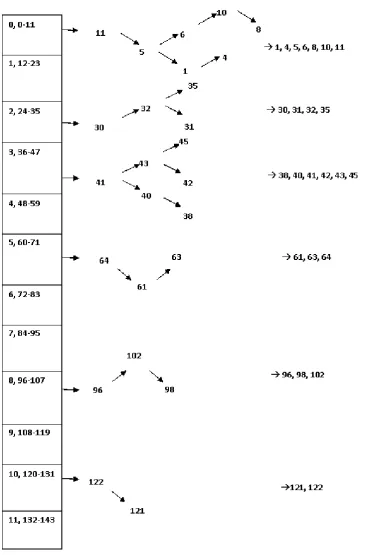
Figure and table on next page demonstrate a complete example solved on a small item set of 25. Unordered set of these 25 values include one, two and three digit number. The problem can be extended to n numbers with maximum digit width as per the capacity of processing environment. Table I gives the complete representation of data items and their corresponding calculated index values as per formulas described. Same data and index values have been represented in the form of complete Indexed Tree in next picture, Figure 3.
4.2 Complexity Analysis
Let T(n) be the time to execute IT_Sort on an array of size n. Examination of present algorithm leads to the following formulation for run time.
Eq.… 1 where n is the number of items and m is the index size such that
Eq. … 1(a) Tmax(n) and Tbuild_index(n) refers to the execution time taken to
calculate maximum element of the list and to create the indexed tree of each element of the list. Since approach used here divides the list into smaller k parts with each part to be read separately, time Tindex_read(k) is calculated by summing
up the individual time taken by m different indexes. In isolation these three time complexity functions for both average and worst case can be summarized as calculated in following equations Eq 2 – Eq 5.
A simple linear algorithm to find the maximum element of the list yields time complexity of n in both average and worst case so complexity remains in order of n only
Eq. … 2
In average case time complexity for building an indexed tree of size m comes out to be m log(m) while for worst case it is m2.
Eq. …3(a)
Eq. …3(b)
Last stage of the complexity calculation deals with the simple accessing of the indexed tree. For this, the results vary with average and worst case. Since present work is concentrated on superior time complexity in worst case, discussion will continue on this track only. As per Eq. 1(a), in maximum cases it comes out to be far less than n which is the only key
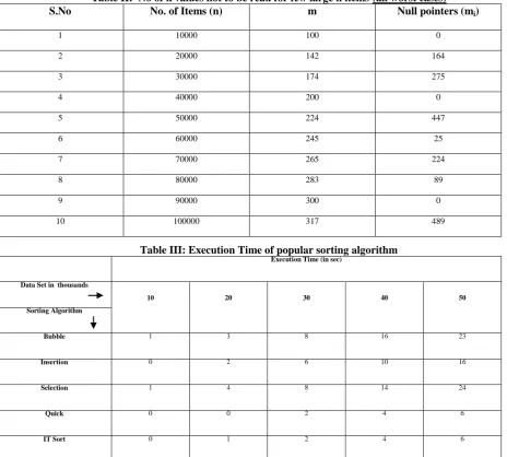
to successful implementation of the algorithm in worst case also. In initial analysis m appears to be very large and deceives with higher complexity issues but even the larger value of m is leading to fewer k’s in Eq 1. Many of the k values are unutilized and not required to be read as per the programming techniques used. Many of the null indexes will remain untouched in actual sort procedure. A demonstration for this has been given in the example considered in previous part (Figure 3). In order to substantiate the fact, Table II illustrates the difference between the n and m2as number of null pointers.This huge difference in these random values can portrait any maximum n and corresponding m value.
There will be one mi associated with each Tindex_read(k) for k
varying from 1 to m whose value can be any integer greater than or equal to 0 which will be deducted every time Tindex_read(k) is calculated. Above revealed Tabular results are
for worst case only where all maximum 100000 values are there in the list in decreasing order. Number of null pointers will increase drastically with average cases where data set will have a normal range of random numbers. This time extraction λ is responsible for decreasing the complexity in worst case with very huge data set and large values.
Formally, λ can be defined as total number of null pointers available in the entire indexed tree.
Eq …. 4
Using Eq 3(a), and Eq. 3(b), for both worst case and average case
Eq. … 5
Complexity comes out to be O(n) Putting the results of Eq 2, 3(b) and 5 for worst case together in Eq. 1, Overall Time Complexity:
Or
Similarly, combining the results of Eq 2, 3(a) and 5 for average case together in Eq. 1,
Or
Table I: Index value of randomly selected 25 data items
Item N Value Index
1 30 2
2 122 11
3 96 8
4 64 5
5 41 3
6 43 3
7 121 11
8 32 2
9 11 0
10 5 0
11 61 5
12 40 3
13 6 0
14 38 3
15 102 8
16 45 3
17 10 0
18 98 8
19 63 5
20 35 2
21 8 0
22 42 3
Table II: No of k values not to be read for few large n items (all worst cases)
S.No No. of Items (n) m Null pointers (mi)
1 10000 100 0
2 20000 142 164
3 30000 174 275
4 40000 200 0
5 50000 224 447
6 60000 245 25
7 70000 265 224
8 80000 283 89
9 90000 300 0
10 100000 317 489
Table III: Execution Time of popular sorting algorithm Execution Time (in sec)
Data Set in thousands
10 20 30 40 50
Sorting Algorithm
Bubble 1 3 8 16 23
Insertion 0 2 6 10 16
Selection 1 4 8 14 24
Quick 0 0 2 4 6
IT Sort 0 1 2 4 6
5. CONCLUSION AND FUTURE WORK
The above discussion and experimental results contribute in making a conclusion that IT Sort perform much better in comparisons to most of the widely used popular sorting algorithms. Time complexity can be reduced with grouping and arranging data in separate Indexed Trees. The same experiment can be extended to parallel environment with multi processor architectures. All different Indexed Trees can be created on separate processor and manipulations can be done simultaneously in each processor. It will further reduce execution time. Our next paper in this series would be
[3] Liu C. L., Analysis of sorting algorithms, Proceedings of Switching and Automata Theory, 12th Annual Symposium, 1971, East Lansing, MI, USA, pp 207-215 [4] Zulkarnain Md. Ali, Reduce Computation Steps Can
Increase the Efficiency of Computation Algorithm, Journal of Computer Science 6, 1203-1207, 2010 [5] Brian W. Kernighan, Dennis M. Ritchie, The C
Programming Language