A Novel Class Imbalance Learning using Ordering
Points Clustering
K. Nageswara Rao
Research Scholar Dept of Comp.sci&EngineeringGITAM UNIVERSITY Visakhapatnam
T. Venkateswara Rao
Phd, ProfessorDept of Comp.sci&Engineering KL UNIVERSITY
Vijayawada
D. Rajya Lakshmi
Phd, Professor Dept of Info. TechnologyGITAM UNIVERSITY Visakhapatnam
ABSTRACT
In Data mining and Knowledge Discovery hidden and valuable knowledge from the data sources is discovered. The traditional algorithms used for knowledge discovery are bottle necked due to wide range of data sources availability. Class imbalance is a one of the problem arises due to data source which provide unequal class i.e. examples of one class in a training data set vastly outnumber examples of the other class(es).This paper proposes a method belonging to under sampling approach which uses OPTICS one of the best visualization clustering technique for handling class imbalance problem. In the proposed approach, further Classification of new data is performed by applying C4.5 algorithm as the base algorithm. The method is optimized by the selection of the most suitable clusters for deletion of the majority dataset based on visualization algorithms. An experimental analysis is carried out over a wide range of highly imbalanced data sets and uses the statistical tests suggested in the specialized literature. The results obtained show that our novel proposal outperforms other classic and recent models in terms of Area under the ROC Curve, F-measure, precision, TP rate and TN rate.
Index Terms— Classification, class imbalance, CIL-OP.
1. INTRODUCTION
Unbalanced dataset learning is a new paradigm of machine learning which has applicability in real time, since all the datasets of real time are of unbalanced nature. For example if you consider a case of medical surgery or scientific experimental analysis the cases in this study will not be of balanced category. The cases may be more in either positive category or negative category, thereby creating an unbalanced dataset. Unbalanced data set is that samples of some classes in the data set are more than samples of other classes, classes with more samples are called majority class, on the other hand, classes with a few samples are called minority class[1]. In the case of unbalanced datasets the common shortcoming using traditional classifiers is that they misclassify minority dataset as majority dataset. In real time scenario this misclassification will cost a lot to the area of applicability in terms of money if it is banking domain, in terms of life if it is medical domain, in terms of quality if it is quality control domain etc. In real time domain the classification accuracy of minority class is as equal as classification accuracy of majority class. There is an urgent need to improve the classificatory performance of minority class in the fields of machine learning and pattern recognition.
To solve the problem of class imbalance the focus is on developing three approaches. First approach is algorithmic development, which lay more stress on developing novel
algorithms which can efficiently handle imbalanced dataset without any loss of generality. Second approach is data level approach, which focuses on preprocessing the data so as to make it balanced. This approach has some advantages of being algorithm independent, data concentric etc over the first approach. Third approach is the hybrid approach, which uses both algorithmic level and data level approaches to solve the problem of unbalanced datasets.
In this work, we focus on imbalanced binary classification problems, having selected a benchmark of 10 datasets from UCI machine learning repository [2]. We perform our experimental study focusing on the precision, F-measure, TP Rate, TN Rate of the models using the Area under the ROC curve (AUC). On the other hand, after comparing these techniques we also want to find what is the source where the difficulties for imbalanced classification emerge. Many other studies on the behavior of several standard classifiers in imbalance domains have shown that significant loss of performance is mainly due to skew of class distributions. However, several investigations also suggest that there are other factors that contribute to such performance degradation, for example, size of the dataset, class imbalance level, small disjoints, density, and overlap complexity[3][4]. This work focuses on the analysis of two of the most
pressing open problems related to data intrinsic
characteristics: overlap and dataset shift.
This paper is organized as follows: first, Section 2 presents the literature survey relating to problem of imbalanced datasets whereas Section 3 describes the proposed approach and its different components. Next, Section 4 describes selected benchmark datasets and the configuration of the methods used in the study. Section 5describes the experimental setting used and different algorithms used for comparison. Section 6 is devoted to discuss the results of our approach and different problem characteristics that make that problem difficult. The conclusions of this work can be found in Section 7.
2. LITERATURE SURVEY ON
IMBALANCE DATASETS
T. Jo et al. [5] have proposed a clustering-based sampling method for handling class imbalance problem, while S. Zouet al. [6] have proposed a genetic algorithm based sampling method. Jinguha Wang et al. [7] have suggested a method for extracting minimum positive and maximum negative features (in terms of absolute value) for imbalanced binary classification is proposed. They have developed two models to yield the feature extractors. Model 1 first generates a set of candidate extractors that can minimize the positive features to be zero, and then chooses the ones among these candidates that can maximize the negative features. Model 2 first generates a set of candidate extractors that can maximize the negative features, and then chooses the ones that can minimize the positive features. Compared with the traditional feature extraction methods and classifiers, the proposed models are less likely affected by the imbalance of the dataset.
Iain Brown et al. [8] have explored the suitability of gradient boosting, least square support vector machines and random forests for imbalanced credit scoring data sets such as loan default prediction. They progressively increase class imbalance in each of these data sets by randomly under sampling the minority class of defaulters, so as to identify to what extent the predictive power of the respective techniques is adversely affected. They have given the suggestion for applying the random forest and gradient boosting classifiers for better performance. Salvador Garcı´aet al. [9] have used evolutionary technique to solve the class imbalance problem. They proposed a method belonging to the family of the nested generalized exemplar that accomplishes learning by storing objects in Euclidean n-space. Classification of new data is performed by computing their distance to the nearest generalized exemplar. The method is optimized by the selection of the most suitable generalized exemplars based on evolutionary algorithms.
Jin Xiao et al. [10] have proposed a dynamic classifier ensemble method for imbalanced data (DCEID) by combining ensemble learning with cost-sensitive learning. In this for each test instance, it can adaptively select out the more appropriate one from the two kinds of dynamic ensemble approach: dynamic classifier selection (DCS) and dynamic ensemble selection (DES). Meanwhile, new cost-sensitive selection criteria for DCS and DES are constructed respectively to improve the classification ability for imbalanced data. Victoria Lópezet al. [11] have analyzed the performance of data level proposals against algorithm level proposals focusing in cost-sensitive models and versus a hybrid procedure that combines those two approaches. They also lead to a point of discussion about the data intrinsic characteristics of the imbalanced classification problem which will help to follow new paths that can lead to the improvement of current models mainly focusing on class overlap and dataset shift in imbalanced classification.
Yang Yong [12] has proposed one kind minority kind of sample sampling method based on the K-means cluster and the genetic algorithm. They used K-means algorithm to cluster and group the minority kind of sample, and in each cluster they use the genetic algorithm to gain the new sample and to carry on the valid confirmation. Chris Seiffertet al. [13] have examined a new hybrid sampling/boosting algorithm, called RUS-Boost from its individual component AdaBoost and SMOTE-Boost, which is another algorithm that combines boosting and data sampling for learning from skewed training data. V. Garcia et al.[14] have investigated the influence of both the imbalance ratio and the classifier on the performance of several resampling strategies to deal with imbalanced data sets. The study focuses on evaluating how learning is affected when different
resampling algorithms transform the originally imbalanced data into artificially balanced class distributions.
María Dolores Pérez-Godoy et al. [15] have proposed CO2RBFN, a evolutionary cooperative–competitive model for the design of radial-basis function networks which uses both radial-basis function and the evolutionary cooperative-competitive technique on imbalanced domains. CO2RBFN follows the evolutionary cooperative–competitive strategy, where each individual of the population represents an RBF (Gaussian function will be considered as RBF) and the entire population is responsible for the definite solution. This paradigm provides a framework where an individual of the population represents only a part of the solution, competing to survive (since it will be eliminated if its performance is poor) but at the same time cooperating in order to build the whole RBFN, which adequately represents the knowledge about the problem and achieves good generalization for new patterns.
Der-Chiang Li et al. [16] have suggested a strategy which over-samples the minority class and under-over-samples the majority one to balance the datasets. For the majority class, they build up the Gaussian type fuzzy membership function and a-cut to reduce the data size; for the minority class, they used the mega-trend diffusion membership function to generate virtual samples for the class. Furthermore, after balancing the data size of classes, they extended the data attribute dimension into a higher dimension space using classification related information to enhance the classification accuracy. Enhong Cheet al. [17] have described a unique approach to improve text categorization under class imbalance by exploiting the semantic context in text documents. Specifically, they generate new samples of rare classes (categories with relatively small amount of training data) by using global semantic information of classes represented by probabilistic topic models. In this way, the numbers of samples in different categories can become more balanced and the performance of text categorization can be improved using this transformed data set. Indeed, this method is different from traditional re-sampling methods, which try to balance the number of documents in different classes by re-sampling the documents in rare classes. Such re-sampling methods can cause over fitting. Another benefit of this approach is the effective handling of noisy samples. Since all the new samples are generated by topic models, the impact of noisy samples is dramatically reduced.
Alberto Fernándezet al. [18] have proposed an improved version of fuzzy rule based classification systems (FRBCSs) in the framework of imbalanced data-sets by means of a tuning step. Specifically, they adapt the 2-tuples based genetic tuning approach to classification problems showing the good synergy between this method and some FRBCSs. The proposed algorithm uses two learning methods in order to generate the RB for the FRBCS. The first one is the method proposed in [19], that they have named the Chi et al.’s rule generation. The second approach is defined by Ishibuchi and Yamamoto in [20] and it consists of a Fuzzy Hybrid Genetic Based Machine Learning (FH-GBML) algorithm.
random forests, as a cost-sensitive learner, performs significantly better compared to random forests.
Che-Chang Hsu et al. [22] have proposed a method with a model assessment of the interplay between various classification decisions using probability, corresponding decision costs, and quadratic program of optimal margin classifier called: Bayesian Support Vector Machines (BSVMs) learning strategy. The purpose of their learning method is to lead an attractive pragmatic expansion scheme of the Bayesian approach to assess how well it is aligned with the class imbalance problem. In the framewor5k, they did modify in the objects and conditions of primal problem to reproduce an appropriate learning rule for an observation sample.
In [23] Alberto Fernándezet al. have proposed to work with fuzzy rule based classification systems using a preprocessing step in order to deal with the class imbalance. Their aim is to analyze the behavior of fuzzy rule based classification systems in the framework of imbalanced data-sets by means of the application of an adaptive inference system with parametric conjunction operators.Jordan M. Malofet al.[24] have empirically investigates how class imbalance in the available set of training cases can impact the performance of the resulting classifier as well as properties of the selected set. In this K-Nearest Neighbor (k-NN) classifier is used which is a well-known classifier and has been used in numerous case-based classification studies of imbalance datasets.
Haibo Heet al.[25] have provided a comprehensive review of the development of research in learning from imbalanced data. Their focus is to provide a critical review of the nature of the problem, the state-of-the-art technologies, and the current assessment metrics used to evaluate learning performance under the imbalanced learning scenario. Yok-Yen Nguwiet al. [26] have proposed a model which uses support vector machines and Emergent Self Organization Map (ESOM) to overcome the problem of class imbalance learning. Their proposed methodology is similar to the algorithmic approach which comprises of the support vector machine (SVM)based criterion ranking feature selection and Emergent Self-Organizing Mapping (ESOM) for unsupervised classification. The input data are first trained by SVM classifier and the ranking criterion are evaluated for feature ranking. The data are then clustered by the ESOM algorithm and such clusters are assigned for classification.
Bao-Liang LUet al. [27] have proposed a Min-Max modular support vector machine (M3-SVM), which approaches this problem by decomposing the training input sets of the majority classes into subsets of similar size and pairing them into balanced two-class classification sub problems. This approach has the merits of using general classifiers, incorporating prior knowledge into task decomposition and parallel learning.
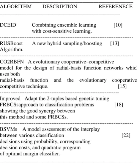
[image:3.595.307.538.87.369.2]Table I presents the recent algorithmic advances in class imbalance learning available in the literature. Obviously, there are many other algorithms which are not included in this table. A profound comparison of the above algorithms and many others can be gathered from the references list.
Table 1Recent Advances in Class Imbalance Learning __________________________________________________ ALGORITHM DESCRIPTION REFERENECE _____________________________________________
DCEID Combining ensemble learning [10] with cost-sensitive learning.
--- RUSBoost A new hybrid sampling/boosting [13] Algorithm.
--- CO2RBFN A evolutionary cooperative–competitive
model for the design of radial-basis function networks which uses both
radial-basis function and the evolutionary cooperative-competitive technique. [15] ---Improved Adapt the 2-tuples based genetic tuning FRBCSsapproach to classification problems [18] showing the good synergy between
this method and some FRBCSs.
--- BSVMs A model assessment of the interplay
between various classification [22] decisions using probability, corresponding
decision costs, and quadratic program of optimal margin classifier.
__________________________________________________
3. CLASS IMBALANCE LEARNING
USING ORDER POINT CLUSTERING
In this section, we follow a design decomposition approach to systematically analyze the different unbalanced domains. We first briefly introduce the design decomposition methodology adopted for new proposed approach.
Algorithm 1:CILOP
1: {Input: A set of minor class examples
P
, a set
Of major class examples
N
,
jPj<jN j}
2: Apply OPTICS on N.
3: Identify Clusters i from N
4: Delete minority class clusters from i and
form Ni.
5: Combine P and Ni to form NPi
6:Train and Learn A Base Classifier (C4.5)
Using NPi.
7: Obtain the values of AUC,TP,FP,F-Measure
OPTICS works on principle like such an extended DBSCAN algorithm for an infinite number of distance parameters which are smaller than a “generating distance”. The only difference is that, in OPTICS assign cluster memberships is not possible. Instead, the order in which the objects are processed is stored and the information which would be used by an extended DBSCAN algorithm to assign cluster memberships (if this were at all possible for an infinite number of parameters). This information consists of only two values for each object: the “core-distance” and a “reachability-distance”.
OPTICS creates an ordering of a database, additionally storing the core-distance and a suitable reachability-distance for each object. This information is sufficient to extract all density-based clustering’s with respect to any distance e’ which is smaller than the generating distance e from this order.
The different components of our proposed algorithm are elaborated in the next subsections.
3.1. Partitioning majority and minority
classes
The unbalanced dataset is partitioned as majority and minority subsets. Since, our approach is a under sampling approach, we need to focus on the majority dataset.
3.2 Applying Clustering Algorithm on
majority class
In the next phase of the approach, we need to apply a clustering algorithm on the majority dataset to identify different clusters. Here we have considered OPTICS clustering algorithm to apply on the majority subset.
3.3 Identification of Minor cluster
sThe result of OPTICS (Ordering Points To Identify Clustering Structure) clustering algorithms is used for identification of number of clusters in the majority subset. We need to identify the weak or outlier clusters and delete those from the majority subset. The amount of deletion will depend upon the unique properties of the dataset. After removing weak and outlier clusters form a new majority subset Ni.
3.4. Forming new balanced dataset
The new majority subset Ni and the minority subset P are combined to form a new likely balanced dataset. This newly formed balanced dataset is applied to a base algorithm; in this case C4.5 is used to obtain different measures such as AUC, Precision, F-measure, TP Rate and TN Rate.
4. DATASETS AND MEASURES
We considered Ten benchmark real-world imbalanced dataset from the UCI machine learning repository [2] to validate our proposed method. Table I summarizes the details of these datasets in the ascending order of the positive-to-negative dataset ratio. This contains the name of the dataset, the total number of examples (Total), attribute, the number of target classes for each dataset, number of minority class examples (#min.), the number of .majority class examples (#maj.). These
datasets represent a whole variety of domains, complexities, and imbalance ratios.
For every data set, we perform a tenfold stratified cross validation. Within each fold, the classification method is repeated ten times considering that the sampling of subsets introduces randomness. The AUC, Precision, F-measure, TP rate and TN Rate of this cross-validation process are averaged from these ten runs. The whole cross-validation process is repeated for ten times, and the final values from this method are the averages of these ten cross-validation runs.
Evaluation Criteria:
To assess the classification results we count the number of true positive (TP),true negative (TN), false positive (FP) (actually negative, but classified as positive) and false negative (FN) (actually positive, but classified as negative) examples. It is now well known that error rate is not an appropriate evaluation criterion when there is class imbalance or unequal costs. In this paper, we use AUC, Precision, F-measure, TP Rate and TN Rate as performance evaluation measures.
Let us define a few well known and widely used measures: Apart from these simple metrics, it is possible to encounter several more complex evaluation measures that have been used in different practical domains. One of the most popular techniques for the evaluation of classifiers in imbalanced problems is the Receiver Operating Characteristic (ROC) curve, which is a tool for visualizing, organizing and selecting classifiers based on their tradeoffs between benefits (true positives) and costs (false positives).
The most commonly used empirical measure, accuracy does not distinguish between the number of correct labels of different classes, which in the framework of imbalanced problems may lead to erroneous conclusions. For example a classifier that obtains an
Accuracy of 90% in a dataset with a degree of imbalance 9:1, might not be accurate if it does not cover correctly any minority class instance.
Because of this, instead of using accuracy, more correct metrics are considered. A quantitative representation of a ROC curve is the area under it, which is known as AUC. When only one run is available from a classifier, the AUC can be computed as the arithmetic mean (macro-average) of TP rate and TNrate:
The Area under Curve (AUC) measure is computed by,
Or
2
1
TP
RATEFP
RATEAUC
2
RATE RATE
TN
TP
AUC
FN
FP
FN
TP
TN
TP
ACC
On the other hand, in several problems we are especially interested in obtaining high performance on only one class. For example, in the diagnosis of a rare disease, one of the most important things is to know how reliable a positive diagnosis is. For such problems, the precision (or purity) metric is often adopted, which
can be defined as the percentage of examples that are correctly labeled as positive:
The Precision measure is computed by,
TP FP TP ecision Pr
The F-measure Value is computed by,
To deal with class imbalance, sensitivity (or recall) and specificity have usually been adopted to monitor the classification performance on each class separately. Note that sensitivity (also called true positive rate, TP rate) is the percentage of positive examples that are correctly classified, while specificity (also referred to as true negative rate, TN rate) is defined as the proportion of negative examples that are correctly classified:
The True Positive Rate measure is computed by,
TP FN TP veRateTruePositi
The True Negative Rate measure is computed by,
TN FP TN veRateTrueNegati
5. EXPERIMENTAL SETTINGS
A
. Algorithms and Parameters
In first place, we need to define a baseline classifier which we use in our proposed algorithm implementation. With this goal, we have used C4.5 decision tree generating algorithm [28]. Furthermore, it has been widely used to deal with imbalanced data-sets [26]–[28], and C4.5 has also been included as one of
the top-ten data-mining algorithms [29]. Because of these facts, we have chosen it as the most appropriate base learner. C4.5 learning algorithm constructs the decision tree top-down by the usage of the normalized information gain (difference in entropy) that results from choosing an attribute for splitting the data. The attribute with the highest normalized information gain is the one used to make the decision.
To validate the proposed CILOP algorithm, we compared it with the traditional C4.5,CART,REP and SMOTE. Eleven real world benchmark data sets taken from the UCI Machine Learning Repository are used throughout the experiments (see Table 1). We performed the implementation using Weka on Windows XP with 2Duo CPU running on 3.16 GHz PC with 3.25 GB RAM.
B. Evaluations on Ten Real-World Datasets:
We evaluate the CILOP model on ten real-world datasets obtained from the University of California at Irvine machine learning repository [2].
[image:5.595.306.532.363.502.2]We then construct classifiers from the imbalanced data based on the training dataset, and perform evaluations on the test data. We repeat this procedure ten times and use the average of the results as the performance metric. The detailed information about the datasets is described in Table 2.
Table 2 Summary of benchmark imbalanced data sets __________________________________________________ Datasets # Ex.# Atts. Class (_,+)
__________________________________________________ Ecolic 336 8 (cp, im)
Hepatitis 155 19 (die; live) Ionosphere 351 34 (b;g) Labor 56 16 (bad ; good ) Breast_w 699 9 (benign; malignant) Colic 368 23 (yes, no)
Diabetes 768 8 (tested-positive; tested-negative) Vote 435 16 (democrat ;republican ) Sonar 208 61 (Rock, Mine)
Sick 3772 30 (Negative, Sick)
__________________________________________________
6. EXPERIMENTAL RESULTS
We have analysis the performance of our proposed algorithm CILOP on class imbalance problem on the following tenreal-world datasets.
The results of the tenfold cross validation with standard deviation are shown in Table 3 to 12.Tables 13-17, we can observe the results of our proposed algorithm CILOP Vs various algorithms with respect to AUC, Precision, F-measure, TP rate and TN rate.
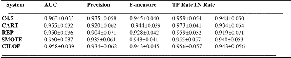
Table 3 Tenfold cross validation classification performance for Ecolic dataset
System AUC Precision F-measure TP Rate TN Rate
_____________________________________________________________________________________________
C4.5 0.963±0.033 0.935±0.058 0.945±0.040 0.959±0.054 0.948±0.050
CART 0.955±0.032 0.920±0.062 0.944±0.039 0.973±0.041 0.934±0.054
REP 0.950±0.036 0.904±0.071 0.928±0.042 0.959±0.052 0.919±0.071
SMOTE 0.960±0.037 0.935±0.061 0.943±0.041 0.955±0.057 0.948±0.053
CILOP 0.958±0.039 0.934±0.062 0.943±0.045 0.956±0.057 0.943±0.056
_____________________________________________________________________________________________
call ecision
call ecision
measure F
Re Pr
Re Pr
2
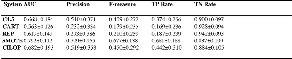
[image:5.595.51.543.672.771.2]Table 4 Tenfold cross validation classification performance for Hepatitis dataset
System AUC Precision F-measure TP Rate TN Rate
C4.5 0.668±0.184 0.510±0.371 0.409±0.272 0.374±0.256 0.900±0.097
CART 0.563±0.126 0.232±0.334 0.179±0.235 0.169±0.236 0.928±0.094
REP 0.619±0.149 0.293±0.386 0.210±0.259 0.187±0.239 0.942±0.093
SMOTE 0.792±0.112 0.709±0.165 0.677±0.138 0.681±0.188 0.837±0.109
CILOP 0.682±0.193 0.519±0.358 0.450±0.292 0.442±0.310 0.884±0.105
Table 5 Tenfold cross validation classification performance for Ionosphere dataset
System AUC Precision F-measure TP Rate TN Rate
C4.5 0.891±0.060 0.895±0.084 0.850±0.066 0.821±0.107 0.940±0.055
CART 0.896±0.059 0.868±0.096 0.841±0.070 0.803±0.112 0.921±0.066
REP 0.902±0.054 0.886±0.092 0.848±0.067 0.826±0.104 0.933±0.063
SMOTE0.904±0.053 0.934±0.049 0.905±0.048 0.881±0.071 0.928±0.057
[image:6.595.51.543.256.353.2]CILOP 0.878±0.076 0.889±0.092 0.849±0.078 0.823±0.110 0.933±0.061
Table 6 Tenfold cross validation performance for labor dataset
_____________________________________________________________________________________________ System AUC Precision F-measure TP Rate TN Rate
_____________________________________________________________________________________________ C4.5 0.726±0.224 0.696±0.359 0.636±0.312 0.640±0.349 0.833±0.127
CART 0.750±0.248 0.715±0.355 0.660±0.316 0.665±0.359 0.871±0.151
REP 0.767±0.232 0.698±0.346 0.650±0.299 0.665±0.334 0.765±0.194
SMOTE 0.833±0.127 0.871±0.151 0.793±0.132 0.765±0.194 0.847±0.187
[image:6.595.51.550.520.616.2]CILOP 0.767±0.219 0.712±0.303 0.699±0.270 0.750±0.322 0.777±0.23
Table 7 Tenfold cross validation classification performance for Breast-w dataset
System AUC Precision F-measure TP Rate TN Rate
C4.5 0.957±0.034 0.965±0.026 0.962±0.021 0.959±0.033 0.932±0.052
CART 0.950±0.032 0.968±0.026 0.959±0.020 0.952±0.034 0.940±0.051
REP 0.957±0.030 0.965±0.030 0.960±0.021 0.957±0.033 0.931±0.060
SMOTE0.967±0.025 0.974±0.024 0.960±0.022 0.947±0.035 0.975±0.024
CILOP 0.953±0.034 0.966±0.036 0.955±0.030 0.946±0.044 0.962±0.042
[image:6.595.53.542.648.743.2]_____________________________________________________________________________________________
Table 8 Tenfold cross validation classification performance for Colic dataset
_____________________________________________________________________________________________ System AUC Precision F-measure TP Rate TN Rate
C4.5 0.843±0.070 0.851±0.051 0.888±0.044 0.931±0.053 0.717±0.119
CART 0.847±0.070 0.853±0.053 0.890±0.040 0.932±0.050 0.720±0.114
REP 0.844±0.067 0.857±0.056 0.882±0.043 0.914±0.066 0.731±0.121
SMOTE0.908±0.040 0.853±0.057 0.880±0.042 0.913±0.058 0.862±0.063
CILOP 0.840±0.067 0.848±0.056 0.885±0.040 0.927±0.048 0.715±0.122
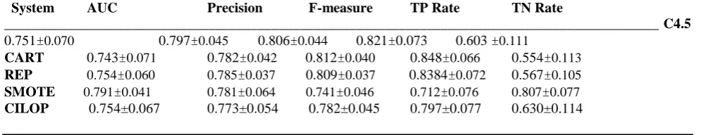
Table 9 Tenfold cross validation classification performance for Pima Diabetes dataset
System AUC Precision F-measure TP Rate TN Rate
_____________________________________________________________________________________________ C4.5
0.751±0.070 0.797±0.045 0.806±0.044 0.821±0.073 0.603 ±0.111
CART 0.743±0.071 0.782±0.042 0.812±0.040 0.848±0.066 0.554±0.113
REP 0.754±0.060 0.785±0.037 0.809±0.037 0.8384±0.072 0.567±0.105
SMOTE 0.791±0.041 0.781±0.064 0.741±0.046 0.712±0.076 0.807±0.077
[image:7.595.53.520.222.313.2]CILOP 0.754±0.067 0.773±0.054 0.782±0.045 0.797±0.077 0.630±0.114
Table 10 Tenfold cross validation performance for vote dataset
____________________________________________________________________________________________ System AUC Precision F-measure TP Rate TN Rate
___________________________________________________________________________________________ C4.5 0.979±0.025 0.971±0.027 0.972±0.021 0.974±0.029 0.953±0.045
CART 0.973±0.027 0.971±0.028 0.966±0.022 0.961±0.037 0.953±0.046
REP 0.957±0.023 0.969±0.035 0.961±0.025 0.955±0.034 0.949±0.059
SMOTE 0.984±0.017 0.977±0.027 0.969±0.021 0.963±0.037 0.981±0.023
CILOP 0.984±0.022 0.964±0.039 0.971±0.027 0.980±0.032 0.952±0.053
[image:7.595.52.525.346.437.2]_____________________________________________________________________________________________
Table 11 Tenfold cross validation performance for Sonar dataset
_____________________________________________________________________________________________ System AUC Precision F-measure TP Rate TN Rate
_____________________________________________________________________________________________
C4.5 0.753±0.113 0.728±0.121 0.716±0.105 0.721±0.140 0.749±0.134
CART 0.721±0.106 0.709±0.118 0.672±0.106 0.652±0.137 0.756±0.121
REP 0.746±0.106 0.733±0.134 0.689±0.136 0.685±0.192 0.762±0.145
SMOTE 0.814±0.090 0.863±0.068 0.861±0.061 0.865±0.090 0.752±0.113
CILOP 0.741±0.115 0.760±0.118 0.737±0.118 0.733±0.159 0.734±0.149
[image:7.595.53.539.466.712.2]______________________________________________________________________________________________________________
Table 12 Tenfold cross validation performance for Sick dataset
_____________________________________________________________________________________________ System AUC Precision F-measure TP Rate TN Rate
_____________________________________________________________________________________________ C4.5 0.726±0.224 0.696±0.359 0.636±0.312 0.640±0.349 0.833±0.127
CART 0.750±0.248 0.715±0.355 0.660±0.316 0.665±0.359 0.871±0.151
REP 0.767±0.232 0.698±0.346 0.650±0.299 0.665±0.334 0.765±0.194
SMOTE 0.833±0.127 0.871±0.151 0.793±0.132 0.765±0.194 0.847±0.187
CILOP 0.959±0.039 0.992±0.004 0.993±0.003 0.994±0.005 0.887±0.064
Fig. 1(a) Fig. 1(b)
0.94 0.96 0.98 1
Vote
C4.5
CART
REP
SMOTE
CILOP
0 0.5 1 1.5
SICK
C4.5
REP
CART
SMOTE
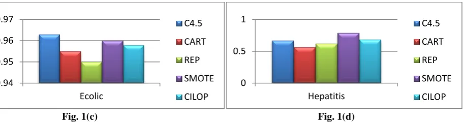
Fig. 1(c) Fig. 1(d)
[image:8.595.65.522.70.192.2]Fig. 1(a) – 1(d) Test results on AUC between the C4.5, CART, REP, SMOTE, and CIL-NN for Hepatitis, Pima Diabetes, Sonar and Sick datasets.
Table 13. Summary of results on AUC Vs CILOP
_____________________________________________
System C4.5 CART REP SMOTE
Dataset __________________________________
Ecolic Loss Win Win Tie
Hepatitis Win Win Win Loss Ionosphere Loss Loss Loss Loss Labor Win Win Tie Loss Breast_w Loss Win Loss Loss Colic Loss Loss Loss Loss Diabetes Win Win Tie Loss Vote Win Win Win Tie Sonar Loss Win Loss Loss Sick Win Win Win Win
[image:8.595.305.511.247.387.2]____________________________________________
Table 14. Summary of results on Precision Vs CILOP
_____________________________________________
System C4.5 CART REP SMOTE
Dataset __________________________________
Ecolic Tie Win Win Tie
Hepatitis Win Win Win Loss Ionosphere Loss Win Win Loss Labor Win Tie Win Loss Breast_w Tie Loss Tie Loss
Colic Loss Loss Loss Loss
Diabetes Loss Loss Loss Loss Vote Loss Loss Loss Loss Sonar Win Win Win Loss Sick Win Win Win Win
[image:8.595.54.275.280.417.2]____________________________________________
Table 15. Summary of results on F-Measure Vs CILOP
_____________________________________________
System C4.5 CART REP SMOTE
Dataset __________________________________
Ecolic Tie Tie Win Tie
Hepatitis Win Win Win Loss Ionosphere Tie Win Tie Loss Labor Win Win Win Loss Breast_w Loss Loss Loss Loss
Colic Loss Loss Win Loss
Diabetes Loss Loss Loss Win Vote Tie Win Win Tie Sonar Win Win Win Loss Sick Win Win Win Win ____________________________________________________
Table 16. Summary of results on TP Rate Vs CILOP _____________________________________________
System C4.5 CART REP SMOTE Dataset __________________________________ Ecolic Loss Loss Loss Tie Hepatitis Win Win Win Loss Ionosphere Win Win Loss Loss Labor Win Win Win Loss Breast_w Loss Loss Loss Tie
Colic Loss Loss Win Win
[image:8.595.308.509.415.550.2]Diabetes Loss Loss Loss Win Vote Win Win Win Win Sonar Win Win Win Loss Sick Win Win Win Win ________________________________________
Table 17. Summary of results on TN Rate Vs CIL-NN _____________________________________________
System C4.5 CART REP SMOTE Dataset __________________________________
Ecolic Loss Win Win Loss
Hepatitis Loss Loss Loss Win Ionosphere Loss Win Tie Win Labor Loss Loss Win Loss Breast_w Win Win Win Loss
Colic Tie Loss Loss Loss
Diabetes Win Win Win Loss Vote Tie Tie Win Loss Sonar Loss Loss Loss Loss Sick Win Win Win Win ____________________________________________
Results on AUC:
From Table 13, one can observe the results of AUC of CILOP against other algorithms. Vote and Sick are one of the two datasets which are of large size (435, 3772). The AUC results for these two datasets are good in terms of wins. The datasets Ecolic,, Hepatitis and Labor have registered some wins and losses too. Ionosphere, Breast_w, Colic and Sonar have not performed well. From Fig 1 (a) – (d) gives the results of Vote, Sick, Ecolic and Hepatitis
Results on Precision:
From Table 14, we can see the results of CILOP against other algorithms, in terms of precision. The datasets Ecolic, Hepatitis, Ionosphere, Labor, Sonar and Sick have performed well, by registering good number of wins. The datasets Breast_w, Colic, Diabetes and Vote have not performed well and have registered less number of wins when compared to C4.5, CART, REP and 0.94
0.95 0.96 0.97
Ecolic
C4.5
CART
REP
SMOTE
CILOP
0 0.5 1
Hepatitis
C4.5
CART
REP
SMOTE
[image:8.595.53.275.451.589.2] [image:8.595.54.275.618.754.2]SMOTE. In overall, from all the Table 14 we can observe that the most of the datasets have performed well on one or the other algorithm. One the Reason for the underperformance of some datasets may be their unique properties such as size, irrelevant attributes present in the dataset.
Results on F-measure:
From the results of Table 15, we can conclude that the datasets Hepatitis, Labor, Vote, Sonar and Sick have shown their performance up to the expectation and had registered good number of wins. The datasets Ecolic and Ionosphere have achieved maximum ties with the existing algorithms in terms of F-measure. The datasets Breast_w, Colic and Diabetes have not given good results.
Results on TP Rate:
From Table 16, one can observe the results of TP Rate. Hepatitis, Labor, Vote, Sonar and Sick are the datasets which have registered good number of wins. The datasets Ecolic, Breast_w and Diabetes have not performed well interms of TP Rate.
Results on TN Rate:
From Table 17, we can see that, in terms of TN Rate the datasets Breast_w, Diabetes and Sick have performed well and have registered good number of wins when compared to C4.5, CART, REP and SMOTE. . The datasets Hepatitis, Labor, Colic and Sonar have not performed well.
In overall, from all the tables we can conclude that our algorithm have given good results when compared to other algorithms. The unique properties of datasets such as size of the dataset, majority, minority ratio and the number of attributes will also effect on the results of our algorithm. The above given results are enough to project the validity of our approach and more deep analysis should be done for further analysis.
7. CONCLUSION:
Class imbalance problem have given a scope for a new paradigm of algorithms in data mining. The traditional and benchmark algorithms are worthwhile for discovering hidden knowledge from the data sources, meanwhile Class imbalance Learning methods can improve the results which are very much critical in real world applications. In this paper we present the class imbalance problem, which exploits the clustering strategy in the unsupervised learning, and implement it with C4.5 as its base learner. Experimental results show that our proposed algorithm performed well in the case of multi class imbalance datasets. In our future work, we will apply our proposed algorithm to more learning tasks, especially high dimensional feature learning tasks.
REFERENCES
[1] WEISS GM.Miningwith rarity: A unifying framework[J]. Chicago,, USA, SIGKDD Explorations, 2004; 6(1): 7-19.
[2] A. Asuncion D. Newman. (2007). UCI Repository of Machine Learning Database (School of Information and Computer Science), Irvine, CA: Univ. of California
[Online]. Available:
http://www.ics.uci.edu/∼mlearn/MLRepository.htm
[3] Prati, R. C., & Batista, G. E. A. P. A. (2004). Class imbalances versus class overlapping: An analysis of a learning system behavior. In Proceedings of Mexican international conference on artificial intelligence (MICAI) (pp. 312–321).
[4] Weiss, G. M., & Provost, F. J. (2003). Learning when training data are costly: The effect of class distribution on tree induction. Journal of Artificial Intelligence Research, 19, 315–354.
[5] T. Jo and N. Japkowicz, “Class imbalances versus small disjuncts,” ACM SIGKDD Explor. Newslett., vol. 6, no. 1, pp. 40–49, 2004.
[6] S. Zou, Y. Huang, Y. Wang, J. Wang, and C. Zhou, “SVM learning from imbalanced data by GA sampling for protein domain prediction,” in Proc. 9th Int. Conf. Young Comput. Sci., Hunan, China, 2008, pp. 982– 987.
[7] Jinguha Wang, JaneYou ,QinLi, YongXu,” Extract minimum positive and maximum negative features for imbalanced binary classification”, Pattern Recognition 45 (2012) 1136–1145.
[8] Iain Brown, Christophe Mues, “An experimental comparison of classification algorithms for imbalanced credit scoring data sets”, Expert Systems with Applications 39 (2012) 3446–3453.
[9] Salvador Garcı´a, Joaquı´nDerrac, Isaac Triguero, Cristobal J. Carmona, Francisco Herrera, “Evolutionary-based selection of generalized instances for imbalanced classification”, Knowledge-Based Systems 25 (2012) 3–12. [10] Jin Xiao, Ling Xie, Changzheng He, Xiaoyi Jiang,”
Dynamic classifier ensemble model for customer classification with imbalanced class distribution”, Expert Systems with Applications 39 (2012) 3668–3675.
[11] Victoria López, Alberto Fernández, Jose G. Moreno-Torres, Francisco Herrera, “Analysis of preprocessing vs. cost-sensitive learning for imbalanced classification. Open problems on intrinsic data characteristics”, Expert Systems with Applications 39 (2012) 6585–6608.
[12] Yang Yong, “The Research of Imbalanced Data Set of Sample Sampling Method Based on K-Means Cluster and Genetic Algorithm”, Energy Procedia 17 ( 2012 ) 164 – 170.
[13] Chris Seiffert, Taghi M. Khoshgoftaar, Jason Van Hulse, and Amri Napolitano,” RUSBoost: A Hybrid Approach to Alleviating Class Imbalance”, IEEE TRANSACTIONS ON SYSTEMS, MAN, AND CYBERNETICS—PART A: SYSTEMS AND HUMANS, VOL. 40, NO. 1, JANUARY 2010 185.
[14] V. Garcia, J.S. Sanchez , R.A. Mollineda,” On the effectiveness of preprocessing methods when dealing with different levels of class imbalance”, Knowledge-Based Systems 25 (2012) 13–21.
[15] María Dolores Pérez-Godoy, Alberto Fernández, Antonio Jesús Rivera, María José del Jesus,” Analysis of an evolutionary RBFN design algorithm, CO2RBFN, for imbalanced data sets”, Pattern Recognition Letters 31 (2010) 2375–2388.
sets”, Computers in Biology and Medicine 40 (2010) 509– 518.
[17] EnhongChe, Yanggang Lin, HuiXiong, QimingLuo, Haiping Ma,” Exploiting probabilistic topic models to improve text categorization under class imbalance”, Information Processing and Management 47 (2011) 202– 214.
[18] Alberto Fernández, María José del Jesus, Francisco Herrera,” On the 2-tuples based genetic tuning performance for fuzzy rule based classification systems in imbalanced data-sets”, Information Sciences 180 (2010) 1268–1291.
[19] Z. Chi, H. Yan, T. Pham, Fuzzy Algorithms with Applications to Image Processing and Pattern Recognition, World Scientific, 1996.
[20] H. Ishibuchi, T. Yamamoto, T. Nakashima, Hybridization of fuzzy GBML approaches for pattern classification problems, IEEE Transactions on System, Man and Cybernetics B 35 (2) (2005) 359–365.
[21] J. Burez, D. Van den Poel,” Handling class imbalance in customer churn prediction”, Expert Systems with Applications 36 (2009) 4626–4636.
[22] Che-Chang Hsu, Kuo-Shong Wang, Shih-Hsing Chang,” Bayesian decision theory for support vector machines: Imbalance measurement and feature optimization”, Expert Systems with Applications 38 (2011) 4698–4704.
[23] Alberto Fernández, María José del Jesus, Francisco Herrera,” On the influence of an adaptive inference system in fuzzy rule based classification systems for imbalanced
data-sets”, Expert Systems with Applications 36 (2009) 9805–9812.
[24] Jordan M. Malof, Maciej A. Mazurowski, Georgia D. Tourassi,” The effect of class imbalance on case selection for case-based classifiers: An empirical study in the context of medical decision support”, Neural Networks 25 (2012) 141–145.
[25] Haibo He, Member, IEEE, and Edwardo A. Garcia, “Learning from Imbalanced Data”, IEEE Transactions on knowledge discovery and engineering , Vol 21, No. 9, September 2009.
[26] Yok-Yen Nguwi, Siu-Yeung Cho, “An unsupervised self-organizing learning with support vector ranking for imbalanced datasets”, Expert Systems with Applications 37 (2010) 8303–8312.
[27] Bao-Liang LU, Xiao-Lin WANG, Yang YANG, Hai ZHAO,” Learning from imbalanced data sets with a Min-Max modular support vector machine”, Front. Electr. Electron. Eng. China 2011, 6(1): 56–71.
[28] J. R. Quinlan, C4.5: Programs for Machine Learning, 1st ed. San Mateo, CA: Morgan Kaufmann Publishers, 1993.