Munich Personal RePEc Archive
Absolute Return Volatility
Cotter, John
University College Dublin
2004
Online at
https://mpra.ub.uni-muenchen.de/3529/
Absolute Return Volatility
JOHN COTTER* University College Dublin
Address for Correspondence: Dr. John Cotter,
Director of the Centre for Financial Markets, Department of Banking and Finance,
University College Dublin, Blackrock,
Co. Dublin, Ireland.
E-mail. [email protected]
Ph. +353 1 716 8900 Fax. +353 1 283 5482
June 9, 2005.
Absolute Return Volatility
The use of absolute return volatility has many modelling benefits says John Cotter. An illustration is given for the market risk measure, minimum capital requirements.
Volatility modelling is a key issue for the finance industry from an academic and
practitioner perspective. This is understandable given the importance that volatility
plays in risk management and the development of accurate risk measures. To
illustrate, successful market risk management requires the use of accurate risk
measures such as minimum capital requirements. These risk measures are
underpinned the input of volatility estimates.1
An important key question thus arises: How do we obtain accurate volatility measures
that can be used in market risk management? This paper addresses this by exploring
the asymptotic and finite sample properties of absolute return volatility. Absolute
return volatility is obtained by aggregating high frequency absolute returns into
relatively low frequency, for example, daily volatility estimates. The use of these
measures is illustrated by obtaining the commonly used market risk measure,
minimum capital requirements. We advocate the use of absolute return volatility
gives desirable time series properties and provides accurate measures of volatility.
We begin by noting that standard risk management practices postulate that market
returns belong to a gaussian distribution. As we know this is not so and leads to
inadequate risk measurement. For example, commonly cited deviations from
normality in financial time series are the existence of fat-tails and of serial correlation
in the volatility series, leading to a bias in minimum capital requirement estimates.2 If
however, volatility can be adequately modelled, the risk manager can filter out these
properties from the returns series leading to a gaussian series. These standardised
gaussian returns allow the risk manager to provide conservative and accurate risk
measures.
1
Minimum capital requirements represent reserves that are used to protect financial firms against losses arising from the volatility of their holdings (see Cotter, 2004; for a discussion).
2
Absolute returns, overlooked in comparison to the use of squared returns, have many
advantages in modelling volatility. First, absolute returns are robust in the presence
of extreme or tail movements (Davidian and Carroll, 1987). Tail returns with their
noted fat-tailed characteristic in financial time series are of particular importance in
market risk management and in associated risk measures such as Value at Risk and
minimum capital requirements. Second, accurate measures of unobservable latent
volatility are obtained from absolute return volatility asymptotically through the
theoretical framework of realised power variation. Moreover, absolute return
volatility gives desirable finite sample properties that are applicable in practice for the
risk manager. In particular, the properties match those found in market returns
including serial correlation and by standardising the return series we eliminate these
features.3 Also, absolute return volatility measurement uses data with the highest
frequency and this is beneficial in getting more precise estimates of risk measures
(Merton, 1980).
The theoretical framework of realised power variation that underpins absolute return
volatility is now outlined. This is followed by an illustration of the use of absolute
return volatility in the calculation of minimum capital requirements for long and short
trading positions on the FTSE100 futures contract.
Realised power variation:
One recent major innovation in the volatility literature has been the employment of
realised power variation where realised volatility converges in probability to
integrated volatility. Accurate model free volatility estimates are thus obtained. This
theory relied on in the continuous time literature results in gaussian return innovations
being a standard assumption of the pricing models presented.
The theoretical developments have evolved in conjunction with vast improvements in
high frequency data allowing the continuous time framework to be realistically
examined in a discrete context. The price process is assumed to follow Brownian
3
motion and allows for accurate estimates of unobservable volatility at the limit.
Discrete approximations of the price process using high frequency data have rm, t = pt -
pt-1/m as the continuously compounded returns with m evenly spaced observations per
day. Brownian motion is generalized to allow the volatility to be random but serially
dependent exhibiting the stylized finding for financial return series of volatility
clustering with fat-tailed unconditional distributions.4
Volatility of this price process as measured by integrated volatility is unobservable.
However, realised power variation that incorporates realised absolute variation,
namely the sum of absolute realisations, |rm|, of a process captured at very fine
intervals equate with integrated volatility. This theory of realised power variation
given in Barndorff-Nielsen and Shephard (2003) and Barndorff-Nielsen et al (2003)
extends the framework of quadratic variation presented for different square powers.5
Thus for returns that are white noise and σ2t with continuous sample paths, the
limiting difference between the unobserved volatility estimate and the realised
observed absolute variation is zero.
Barndorff-Nielsen and Shephard (2003) and Barndorff-Nielsen et al (2003) show that
when the framework is for limiting intervals with m →∞, and with power variations,
0.5 > n < 3, realised power variation converges in probability to integrated volatility.
p m d r
t H t
m t j m j m
lim , /
,...,
→ ∞
− +
=
− =
σ τ
τ
2
1
0
| | (1)
Implying for m sampling frequency, the realized absolute variation is consistent with
integrated volatility. Asymptotically the returns process scaled by realised power
variation is normally distributed, N (0, 1).
4
A number of semi-martingales can be utilised, and volatility modelling in this way allow for any number of characteristics documented for financial time series such as long memory and non-stationarity.
5
The use of squared returns relying on quadratic variation has become a tour de force in the recent volatility literature with many studies completed. A flavour of the use of these related measures and a synopsis of the prevailing literature is in Andersen et al (2003). Similar to realised power variation the theory of quadratic variation implies that after assuming sample returns are white noise and σ2
t has
Notwithstanding the derivation of the limiting distribution, our interest in the
modelling process for risk measurement is in terms of its ability to capture financial
return finite-sample properties. Thus, the finite-sample properties and their
consequences especially for relatively small samples that match the investment
horizon of risk managers need exploration.
The practical implementation of the theory simplifies into developing volatility
estimators using aggregated absolute returns, |rm| and its’ variants for any day t with
m intraday intervals:
| |rt |rm t, j m/ |
j m
= +
=1
(2)
For n = 2, this represents the quadratic variation result where squared returns are
equated to integrated volatility.
The number of intervals chosen is asset dependent impacted on by such factors as
levels of trading activity and of inherent volatility. However, there is a trade-off as m
increases the precision of realized power variation increases but microstructure effects
such as bid-ask bounce increasing at finer intervals can impair the modelling process.
This study follows the standard interval choice of 5-minute intervals throughout the
trading day.
As well as directly comparing different volatility series using absolute and squared
reaslisations the study examines the ability of the respective measures to filter out the
time-varying dynamics associated with asset prices. Daily Returns, rt, obtained by
aggregating the high frequency intraday returns, rm, t, are rescaled by the respective
daily volatility series:
zt = rt/σt
where the standardised returns series, zt, are obtained from scaling returns, rt, with
Characteristics of volatility series:
Turning to the application of this method we take high frequency prices for the
FTSE100 futures contract traded on LIFFE, for a relatively short time frame between
January 1, 1999 through June 30, 2000 using the most actively traded delivery month
data from a volume crossover procedure. For each 5-minute interval log closing
prices are first differenced to obtain each period’s return. The full trading day is
between 08.35 and 17.35 entailing 107 5-minute intervals. All non-trading periods
and holidays are removed resulting in 375 full trading days for analysis.
Daily returns and daily volatility series are generated from aggregating intraday
values such as absolute returns and power variations across the trading day. In order
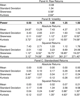
to examine the unconditional distributional properties of the daily return and risk
measures summary statistics are estimated detailing four distributional moments
presented in table 1. A subset of findings for power coefficients between 0.5 and 1.5
are given.6 Also, some distributional plots for the returns series, and the volatility
and standardised returns series with the most attractive distributional characteristics
are given in figure 1. The latter series are of particular interest as we are determining
the extent to which we can filter out the non-gaussian features of financial returns
using the two sets of volatility series.
INSERT TABLE 1 HERE
INSERT FIGURE 1 HERE
The usual finding for the unconditional distribution of financial returns is evident,
namely they are leptokurtotic implying too many realisations bunching around the
peak and tails of the distribution relative to gaussianity. In particular the
distributional plots indicate the fat-tailed characteristic of financial returns with too
many large extreme observations relative to a normal distribution.
In table 1 panel B absolute return volatility and squared return volatility are analysed.
Absolute return volatility clearly dominates squared return volatility in terms of
desirable time series properties. Whilst the coefficients for third and fourth moments
of the volatility series with the most attractive distributional characteristics appear
6
similar, squared returns volatility is more prone to outliers as shown by a very long
right tail in figure 1. In general absolute return volatility is more closely associated to
a normal distribution than squared return volatility at all power transformations.7
The standardised returns series, rescaling daily returns by the different volatility is
presented in panel C. We are interested in determining whether we can obtain
gaussian standardised returns and also identify the volatility processes that allow us to
achieve this aim. We find a positive outcome to this endeavour if we standardise by
absolute volatility only. Thus unconditionally, returns rescaled by absolute return
volatility clearly dominate their squared return counterparts in closely approximating
gaussian features. A number of the standardised returns series rescaled by absolute
returns exhibit no excess skewness and kurtosis and others show a vast improvement
in their characteristics. In fact, the fat-tailed property disappears to the extent that
platykurtotic features exist. These rescaled series can now give appropriate risk
measures that can be extended further, by for example, incorporating the gaussian
square root of time multiplier.
In contrast, the standardised returns rescaled by squared return volatility, with the
exception of [zt] = [rt]/[rt2] 0.50 representing realised standard deviation, still exhibit
strong excess skewness and kurtosis. Interestingly this squared return measure,
realised standard deviation, is equivalent to absolute return volatility, |rt|, and is
equated to unobservable integrated volatility from the theory of realised power
variation.
Other squared return volatility series are unable to capture the dynamics of the returns
series adequately. For instance, the much-used realised variance is unable to remove
the excess kurtosis of the FTSE100 returns series. Thus for relatively small finite
samples it is clear that whilst a spectrum of standardised returns using variants of
absolute returns allow the risk manager to present conservative and accurate risk
measures that adequately model the time-varying dynamics of asset returns this is not
the case for their squared return counterparts.
The theory of realised power variation asymptotically allows the conditional
distribution of volatility to be random but serially dependent and to exhibit the
stylized finding for financial data of volatility clustering. Furthermore, the rescaling
of the returns series by the different volatility proxies should produce a white noise
series devoid of temporal dependence.
To investigate the finite-sample properties of the use of absolute and squared return
volatility and their power variations to match the conditional distribution
characteristics of financial time series, figure 2 presents time series plots and sample
autocorrelation plots for the returns series, volatility and standardised returns series.
The overall finite-sample results suggest that whilst the use of squared realisations
meets only some of the criteria to adequately model financial returns, aggregated
absolute realisations meet all criteria.
INSERT FIGURE 2 HERE
The returns series exhibit time-varying dynamics along with a very large negative
return for August 9, 1999 but is essentially white noise with no significant
dependence for 20 lags.
As seen in table 1 both volatility series have unconditional distributions that are
fat-tailed and in figure 2 both conditional volatility series vary across time and volatility
clusters are clearly evident for the absolute returns series. Volatility clustering is less
evident in the squared returns volatility series as a large outlier dominates it on
August 9 resulting in a single day’s volatility that is more than six times the size of
the next largest realisation. Furthermore, the memory of the volatility series using
absolute realisations indicates strong serial correlation although no such dependence
is evident from using squared realisations, as these are also white noise. Absolute
return volatility thus matches the stylized features of financial time series.
Minimum capital requirements:
Risk managers are interested in the end product of market risk measures such as
standardised returns are now used in to calculate these market risk measures. These
capital reserves protect investors against losses arising from the volatility of their
holdings and thus adequate modeling of volatility is paramount to their accurate
measurement.
Rather than using returns series that would entail an underestimation of risk measures
assuming normality, the gaussian standardized returns are analysed. This allows for
conservative and consistent risk management estimates. These are presented so as to
cover price movements at various probability levels. To illustrate, taking a long
position and expressing the minimum capital requirement Lrmincap as a percentage of
total investment that covers losses Lrloss at a certain probability:
P L[ loss<Lrmincap]=0 95 . (3)
In this case the capital deposit covers 95% of price movements and losses in excess of
this would occur with a 5% frequency. A one-day forecast of the capital required as a
percentage of total investment uses chosen quantiles of the standardized returns
updated with realized volatility measured by
λ
t= −1 exp(|r |t zq) (4)
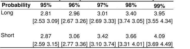
An illustration of minimum capital requirements for long and short trading positions
at common confidence levels is in table 2. For instance, to cover 95% of all price
fluctuations in the FTSE100 contract requires a capital deposit of 2.81% of the total
investment for a long position. Thus this capital outlay would be insufficient for 5%
of the outcomes facing the investor and risk management strategies would be
implemented with these capital costs in mind.
INSERT TABLE 2
In conclusion, this paper advocates alternative measures of volatility using aggregated
absolute returns and their variations. The measures are underpinned by the theory of
realised power variation that asymptotically has absolute variation converging in
probability to the unobservable integrated volatility. The practical use of these
measures is illustrated in the context of minimum capital requirement estimates, a key
The paper shows that the finite-sample properties of absolute return volatility
generally dominate squared return volatility. In particular, rescaling by absolute
return volatility results in gaussian standardised returns for a spectrum of power
variations. Also, volatility clustering and strong serial correlation are evident for
absolute return volatility series matching the properties of financial time series.
Moreover, absolute returns are more robust in the presence of extreme returns that
result in fat-tails. The key to imposing appropriate risk management measures
requires accurate modelling of volatility for different assets. These accurate absolute
return volatility measures are used to give conservative daily minimum capital
References:
Andersen, T. G., T. Bollerslev, and F. X. Diebold (2003). Parametric and
nonparametric measurement of volatility. In Y. Ait-Sahalia and L. P. Hansen (Eds.),
Handbook of Financial Econometrics. Amsterdam: North Holland.
Barndorff-Nielsen, O. E. and N. Shephard (2003). Realised power variation and
stochastic volatility. Bernoulli, 9, 243–265.
Barndorff-Nielsen, O. E. Graversen, S. E., and N. Shephard (2003). Power variation
& stochastic volatility: a review and some new results, Unpublished paper: Nuffield
College, Oxford.
Brooks, C., A. D. Clare and G. Persand, 2002, Estimating market-based minimum
capital risk requirements: A multivariate GARCH approach, Manchester School, 705,
666-681.
Cotter, J., (2004). Minimum Capital Requirement Calculations for UK Futures,
Journal of Futures Markets, 24, 193-220.
Davidian, M., & R. J. Carroll (1987). Variance Function Estimation. Journal of the
American Statistical Association. 82, 1079-1091.
Karatzas, I., & S. E. Shreve, (1991). Brownian Motion and Stochastic Calculus (2nd
ed.). Berlin: Springer-Verlag.
Longin, F.M., (1996). The asymptotic distribution of extreme stock market returns,
Journal of Business, 63, 383-408.
Longin, F.M., (2000). From Value at Risk to Stress Testing: The Extreme Value
Approach Journal of Banking and Finance 24(7), 1097-1130.
Merton R.C., 1980. On Estimating the Expected Return on the Market, Journal of
Financial Economics, 8, 323-361.
Mikosch, T. and C. Starica (2000). Limit theory for the sample autocorrelations and
Table 1: Summary statistics for daily FTSE100 series
Panel A: Raw Returns
Mean -0.08
Standard Deviation 1.34
Skewness 0.58*
Kurtosis 2.64*
Panel B: Volatility
Power 0.50 0.75 1.00 1.25 1.50
Absolute Returns
Mean 24.97 13.29 7.43 4.37 2.71
Standard Deviation 3.43 2.65 2.01 1.63 1.62
Skewness 0.11 0.63* 1.12* 2.23* 6.52*
Kurtosis 3.72* 2.42* 3.12* 10.55* 74.08*
Squared Returns
Mean 7.43 2.71 1.33 1.12 1.76
Standard Deviation 2.01 1.62 3.23 8.69 24.06
Skewness 1.12* 6.52* 16.75* 18.85* 19.23*
Kurtosis 3.12* 74.08* 306.01* 361.21* 371.40*
Panel C: Standardised Returns
Absolute Returns
Mean 0.00 0.00 0.00 0.00 0.00
Standard Deviation 0.05 0.10 0.17 0.29 0.49
Skewness 0.44* 0.22 0.04 0.17 0.24
Kurtosis 2.22* 1.01* -0.12 -0.28 -0.07
Squared Returns
Mean 0.00 0.00 0.02 0.07 0.21
Standard Deviation 0.17 0.49 1.34 3.58 9.58
Skewness 0.04 0.24 0.46* 0.86* 1.30*
Kurtosis -0.12 -0.07 1.35* 4.63* 9.25*
Table 2: Minimum capital requirement estimates for daily FTSE100 series
Probability 95% 96% 97% 98% 99%
Long 2.81 2.96 3.01 3.40 3.95
[2.53 3.09] [2.67 3.26] [2.69 3.33] [3.74 3.05] [3.55 4.34]
Short 2.87 3.06 3.42 3.66 4.09
[2.59 3.15] [2.77 3.36] [3.10 3.74] [3.31 4.01] [3.69 4.49]
Figure 1: Distributional plots for daily FTSE100 series
returns
-10 -5 0 5
0 .0 0 .1 0 0 .2 0 0 .3 0
Quantiles of Standard Normal
re
tu
rn
s
-3 -2 -1 0 1 2 3
-8 -6 -4 -2 0 2
absolute returns ^ 0.75
0 5 10 15 20 25
0 .0 0 .0 5 0 .1 0 0 .1 5
Quantiles of Standard Normal
a b s o lu te r e tu rn s ^ 0 .7 5
-3 -2 -1 0 1 2 3
5 1 0 1 5 2 0 2 5 squared returns
0 20 40 60
0 .0 0 .0 4 0 .0 8 0 .1 2
Quantiles of Standard Normal
s q u a re d r e tu rn s
-3 -2 -1 0 1 2 3
0 1 0 2 0 3 0 4 0 5 0 6 0
standardised absolute returns
-0.6 -0.4 -0.2 0.0 0.2 0.4 0.6
0 .0 0 .5 1 .0 1 .5 2 .0
Quantiles of Standard Normal
s ta n d a rd is e d a b s o lu te r e tu rn s
-3 -2 -1 0 1 2 3
-0 .4 0 .0 0 .4
standardised squared returns ^ 0.75
-1 0 1 2
0 .0 0 .2 0 .4 0 .6
Quantiles of Standard Normal
s ta n d a rd is e d s q u a re d r e tu rn s ^ 0 .7 5
-3 -2 -1 0 1 2 3
-1 .0 0 .0 1 .0
Notes: Density plots followed by q-q plots for the returns, volatility and standardised returns series are presented. The volatility and standardised returns series chosen relying on absolute and squared returns are based on those with the optimal skewness and kurtosis coefficients vis-à-vis normality. Specifically, the volatility series are
|rt|0.75 and [rt2] and the standardised returns series are [zt] = [rt]/|rt| and [zt] =
Figure 2: Time series and Autocorrelation plots for daily FTSE100 series
Jan 1999 - June 2000
re
tu
rn
s
0 100 200 300
-8 -6 -4 -2 0 2 No. Lags A C F r e tu rn s
5 10 15 20
-0 .1 0 -0 .0 5 0 .0 0 .0 5
Jan 1999 - June 2000
a b s o lu te r e tu rn s ^ 0 .7 5
0 100 200 300
5 1 0 1 5 2 0 2 5 No. Lags A C F a b s o lu te r e tu rn s ^ 0 .7 5
5 10 15 20
0 .2 0 .3 0 .4 0 .5 0 .6
Jan 1999 - June 2000
s q u a re d r e tu rn s
0 100 200 300
0 1 0 2 0 3 0 4 0 5 0 6 0 No. Lags A C F s q u a re d r e tu rn s
5 10 15 20
-0 .0 2 0 .0 2 0 .0 6
Jan 1999 - June 2000
s ta n d a rd is e d a b s o lu te r e tu rn s
0 100 200 300
-0 .4 0 .0 0 .4 No. Lags A C F s q u a re d ( s ta n d a rd is e d a b s o lu te r e tu rn s )
500 1000 1500 2000
-0 .0 5 0 .0 0 .0 5 0 .1 0
Jan 1999 - June 2000
s ta n d a rd is e d s q u a re d r e tu rn s ^ 0 .7 5
0 100 200 300
-1 .0 0 .0 1 .0 No. Lags A C F s q u a re d ( s ta n d a rd is e d s q u a re d r e tu rn s ^ 0 .7 5 )
500 1000 1500 2000
-0 .0 5 0 .0 0 .0 5 0 .1 0
Notes: Time series plots followed by ACF plots for the returns, volatility and standardised returns series are presented. The sample autocorrelations are for a displacement of 20 days from a full sample of 375 days with confidence bands of 0.10. The volatility and standardised returns series chosen relying on absolute and squared returns are based on those with the optimal skewness and kurtosis coefficients
vis-à-vis normality. Specifically, the volatility series are |rt|0.75 and [rt2] and the
standardised returns series are [zt] = [rt]/|rt| and [zt] = [rt]/[rt2]0.75. The ACF plots for