Image Compression using FFN for ROI and SPIHT for
background
Vikash Kumar
BIET, Jhansi Jhansi, UP IndiaJitu Sharma
BIET, Jhansi Jhansi, UP India [email protected]Shahanaz Ayub
BIET, Jhansi Jhansi, UP India [email protected]ABSTRACT
The objective of this paper is to develop different method for image compression without reducing the resolution for Region of Interest in the images. Mostly medical images for diagnosis purpose have some specific region; this region is known as Region of Interest (ROI). Here we separate our ROI from background and then apply Feed Forward Neural Network (FFN) compression to ROI and background is compressed using Set Partitioning in Hierarchical Tree (SPIHT) Technique. This paper is in the context to understand the FFN technique which provides low compression by maintaining images resolution of ROI whereas SPIHT technique which gives very high compression ratio for the background. Thus the combination of compressed ROI and compressed background will result in an image with highly compressed background without effecting image resolution of ROI.
General Terms
Image CompressionKeywords
ROI, SPIHT, FFN.1.
INTRODUCTION
There are several imaging devices like ultrasound machine, CT scan which produces high resolution digital medical images of very large size. It’s difficult to store these high resolution images and transmitting them over a transmission channel with limited bandwidth. So there is a need of compression technique which produces digital images without affecting its quality. Image compression can be categorized in two parts (1) Lossless compression (2) lossy compression [1]. Image can be reconstructed exactly the same as the original without any loss of information in Lossless compression, this application is majorly use in medical imagery, where we do not want any loss of important information for analysis purpose [2]. On the other hand in Lossy compression there is some loss of information but it provides high compression ratio of images. Thus, we are going to find a compression technique which gives high compression ratio with acceptable image quality. Now we want a balance between unintentional loss of potential significant information for diagnosis purpose and insufficient reduction that will induce additional cost for larger storage system or sophisticated communication components. The effectiveness of any compression technique is checked by two parameters which are – Compression Ratio (CR) and Mean Square Error (MSE) for accessing the quality of the decompressed image. Equation (1) and (2) gives the mathematical formula for estimating the two parameters.
𝐶𝑅 = 𝑂𝑟𝑖𝑔𝑖𝑛𝑎𝑙 𝐼𝑚𝑎𝑔𝑒 𝐹𝑖𝑙𝑒 𝑆𝑖𝑧𝑒 𝐶𝑜𝑚𝑝𝑟𝑒𝑠𝑠𝑒𝑑 𝐼𝑚𝑎𝑔𝑒 𝐹𝑖𝑙𝑒 𝑆𝑖𝑧𝑒 (1)
𝑀𝑆𝐸 = 1
𝑀 × 𝑁 (𝐹 𝑖, 𝑗 − 𝑓 𝑖, 𝑗 )2 (2)
𝑁−1
𝑗 =0 𝑀−1
𝑖=0
Where F represents original image of size M × N and f is the reconstructed image of same size.
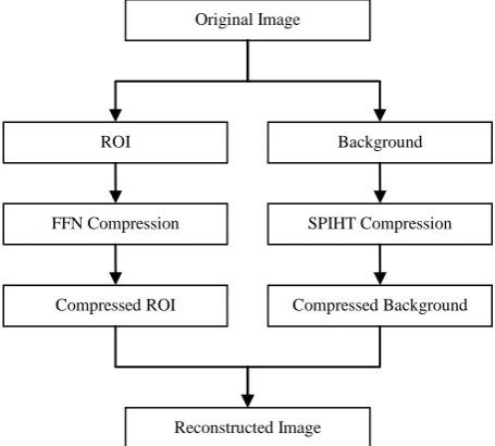
[image:1.595.317.545.493.698.2]The Proposed method could be very useful in compressing medical images of tumors such as in MRI scans for example brain tumor is the region of interest for diagnosis purposes and we do not want any loss of information from that region, so by separating the ROI and applying FFN compression to the ROI we will get lossless reconstructed ROI. Background which is of not much concern can be compressed by SPIHT technique and we achieve a lossy reconstructed background. Merging the reconstructed ROI and background gives a compressed image whose overall compression ratio is very high and the image resolution remains good for any diagnosis purpose.
Figure 1 Block diagram of the compression technique
2.
METHODOLOGY
Here we propose a compression technique in which the original image is first divided into its ROI and background
Original Image
FFN Compression
ROI Background
SPIHT Compression
Compressed Background
[3]. Figure 1 shows the method proposed. Then the ROI is compressed using a feed forward neural network and the background is compressed using set partitioning in hierarchical tree algorithm. The compressed ROI and background are then assembled to obtain the reconstructed image.
2.1
Separation of ROI from Image
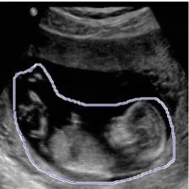
To separate our ROI from image we have used MATLAB 7.12.0 (R2011a) [4]. Many tools are there for selecting ROI but we have used free hand tool so that a user can easily define ROI. Here we have used an ultrasound image for illustration shown in figure 2.
Figure 2 Ultrasound Image
The ROI now can be selected using the free hand tool as shown in figure 3.
Figure 3 Selection of ROI
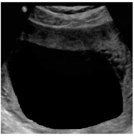
[image:2.595.362.497.84.241.2]Now to separate the ROI we create a mask as shown in figure 4. The mask shown is a binary image where the ROI is filled with 1’s and rest of the image is represented by 0’s. This binary mask cannot be directly used for ROI separation because the original ultrasound image is a gray image where every pixel is represented by a value between 0 and 255. So we have to convert this binary mask to gray image where 1’s are replaced by 255 and there is no change for 0’s. A negative binary mask is also created using the binary mask.
Figure 4 Binary Mask
[image:2.595.99.236.241.379.2]The negative binary mask can be obtained by subtracting the binary mask from 1. The negative binary mask shown in figure 5 is also converted to gray image for obtaining ROI.
Figure 5 Negative Binary Mask
By adding the negative gray mask with the original image we obtain an image shown in figure 6.
[image:2.595.101.235.474.608.2]Thus the ROI can be obtained by just subtracting negative gray mask from figure 6. The ROI is shown in figure 7.
Figure 7 ROI
[image:3.595.360.495.163.377.2]The background can also be separated by similar process. Separated background is shown in figure 8.
Figure 8 Background
2.2
Compression of ROI using FFN
Feed forward neural network compression is similar to JPEG algorithm except the quantization step [5]. In FFN the transformed coefficients are stored in the synaptic weights when learning is complete. FFN also uses Discrete Cosine Transform (DCT) similar to JPEG algorithm. The ROI here is of size 256×256 same as of the original image. This ROI is first converted to sub-images of size 8×8. Thus we have [32×32] =1024 blocks [6].
DCT is applied to each 8×8 sub-images. Dividing the image into sub-images reduces the complexity of the computation and the required memory space. The transformed coefficients with spatial coordinates (x, y) are propagated through FFN block by block sequentially. The spatial coordinates (x, y) are the inputs for the neural network and transformed coefficients are the outputs for the network. There are many algorithms used for training of the network and weight adjustment.
Generally backpropagation algorithm with conjugated gradient technique is used for faster convergence.
The FFN compression technique is still under our study to obtain fast convergence with more compression ratio and acceptable MSE. The block diagram explaining the method is shown in figure 9.
Figure 9 FFN Compression Technique
The main advantage of FFN compression is that it gives compression ratio near to lossy compression technique while MSE is near to lossless compression technique. Thus ROI compressed with this technique has good MSE [5]. In the decompression stage the FFN reproduce each coefficient values with less error.
2.3
Compression of Background by SPIHT
The concept and the implementation of the technique- Set Partitioning in Hierarchical Trees is explained by the flow chart in figure 10. We perform 4 levels of wavelet transform to the background image. Then, this transformed image is given as input to quantization block after which the image is grouped in different ranges of magnitude defined as an integer power of 2. These coefficients are then encoded using the SPIHT technique [7]. The compressed file is then sent to the decoder where it decodes the image using the image decoding SPIHT algorithm. Then, we input the reconstructed image file into the module that will perform inverse wavelet transform. After the inverse wavelet transform is performed we obtain the final reconstructed image. The code was written in MATLAB [4]. For the sake of understanding this rigorous encoding technique, MATLAB [4] was found to be the best available and affordable option.The SPIHT technique produces images with compression ratio of very high order. Background shown in figure 8 is transformed using 4 level wavelet transform. The decomposed image after 4 level transformation is shown in figure 11.
ROI
Sub-images
DCT
FFN
[image:3.595.100.236.352.490.2]Figure 10 SPIHT Compression Technique
Figure 11 Decomposed Background
The reconstructed background image is shown in figure 12.
Figure 12 Reconstructed Background
[image:4.595.332.527.72.265.2]The effectiveness of this compression ratio can be estimated by following table 1.
Table 1 Performance of SPIHT for the ultrasound 256×256 gray image
Parameters Values
MSE 8.8003
PSNR 38.69 dB
Compression ratio 12.7392
Saving of memory 91.67 %
3.
CONCLUSION
The compression ratio obtained by SPIHT technique for the background compression is very high and FFN compression results in good quality images, by which our ROI is compressed. So overall compression ratio of the image will be very high and the image resolution remains good for any diagnosis purpose. This technique can find its application for compressing medical images.
Background Image
Wavelet Transform
Quantization
Encoding
Transmission
Decoding
Inverse Wavelet Transform
[image:4.595.55.280.370.591.2]4.
REFERENCES
[1] R. C. Gonzalez and R. E. Woods, “Digital Image Processing”, Addision Wesley, New York, USA, 1981.
[2] Janaki. R, Tamilarasi. A, “Enhanced ROI (Region of Interest Algorithms) for Medical Image Compression”, International Journal of Computer Applications (0975 – 8887), Volume 38– No.2, pp.38-43, January 2012
[3] Yao He, Ling Tong, Mingquan Jia, “A Compression Image Method Combining Wavelet Transform with SVD”, ICCP 2011 Proceedings.
[4] MATLAB, MATHWORKS INC., MATLAB7.12.0 (R2011a).
[5] W. K. Yeo, David F. W. Yap, K. C. Lim, Andito D.P., M. K. Suaidi, T. H. Oh, “A Feed Forward Neural Network Compression with Near to Lossless Image Quality and Lossy Compression Ratio”, Proceedings of 2010 IEEE Student Conference on Research and Development (SCOReD 2010), 13 - 14 Dec 2010, Putrajaya, Malaysia
[6] Dipta Pratim Dutta, Samrat Deb Choudhury, Md. Anwar Hussain, Swanirbhar Majumder, “Digital Image Compression using Neural Networks”, 2009 ICACCTT.