A Bi-fuzzy Approach to a
Production-Recycling-Disposal Inventory Problem
with Environment Pollution Cost via Genetic
Algorithm
D. K. Jana
Department of Applied Science Haldia Institute of Technology, Haldia, Purba Midna Pur-721657,India
K. Maity
Department of Mathematics Mugberia Gangadhar Mahavidyalaya, Bhupatinagar, Purba Medinipur-721425, W.B.,India
T. K. Roy
Department of Mathematics Bengal Engineering& Science
University, Howrah, India
ABSTRACT
This paper develops a production, recycling-disposal inventory problem over a finite time horizon in fuzzy and bi-fuzzy environ-ments. The production and recycling process are performed in a plant which is located very near to the market. The products of the plant are continuously transfer to the market. Here, the dynamic demand is satisfied by production and recycling. The use units are collected continuously from the customers and then either recycled or disposed. Recycling products can be used as new products which are sold again in the market. The rate of production, recycling and disposal are assumed to be function of time. The setup cost, idle cost and environment pollution recovery cost for production-recycling system in industry are also included. The optimum results are presented both in tabular form and graphically.
Keywords:
Production, Recycling-Disposal, Idle cost, Environment pollu-tion cost, Bi-fuzzyifx
1. INTRODUCTION
During the last few decades, production-recycling system is an important area of inventory studies due to growing envi-ronmental concern and envienvi-ronmental regulations like ’Kyoto Protocol’in industry. Fig-3 represents a single plant production-recycling-disposal system in fuzzy and bi-fuzzy environments. Some units are bought back from market for a recoverable inventory after using by the customers. The serviceable stock is delivered to the customer demand. The serviceable stock can be satisfied by either production or by recycling. The non-recycling items are disposed. The non-serviceable stock is filled up by used products from the customers. The non-serviceable stock is supplied for either recycling or disposal. A number of research papers have already been published on the above type of models by (cf. Minner and Kleber (2001), Dobos and Richter (2006), Maity et al.(2009), Ilgin and Gupta(2010), Taleizadeh et. al. (2012) and others).
In the classical inventory models, normally static lot size models are formulated. But in the manufacturing environment, the static models are not adequate in analyzing the behavior of such systems and in deriving the policies for their control. Moreover
it is usually observed in the market that sales of the fashionable goods, electronic gadgets, seasonable products, food grains, etc., increases with time. For these reasons, dynamic models of production inventory systems have been considered and solved by some researchers (cf. Giri and Chaudhuri (1998), Maity and Maiti (2005a) and others). In these models, demand is assumed to be continuous functions of time and till now, only a very few researchers (cf. Maity and Maiti (2005b)) have taken time dependent production function.
over conventional optimization methods. Holland was inspired by Darwin’s theory about evolution and constructed GAs based upon the fundamental principle of the theory: ‘Survival of the fittest’. The theoretical basis for the GA is the Schema Theorem which states that individual chromosomes with short, low-order, highly fit schemata or building blocks receive an exponentially increasing number of trials in successive generations. In natural genesis, we know that chromosomes are the main carriers of hereditary information from parent to offspring and that genes, which present hereditary factors, are lined up on chromosomes. At the time of reproduction, crossover and mutation take place among the chromosomes of parents. In this way hereditary factors of parents are mixed-up and carried to their offsprings. Again according to Darwinian principle, only the fittest animals can survive in nature. So a pair of fittest parent normally reproduces a better offspring.
In this paper, the production and disposal rates are function of time and unknown taken as control variables. Moreover, the re-cycling rate is unknown constant and control variable. Here, production cost is greater than the recycling cost. Also non-serviceable holding cost is less than non-serviceable holding cost. The total cost is minimized and solved by genetic algorithm technique. None has considered a plants production, recycling-disposal inventory problem in fuzzy and bi-fuzzy environments. The optimum production, recycling-disposal and stock levels are determined for known dynamic demand function. The model is illustrated through numerical examples and results are also pre-sented graphically.
2. NECESSARY KNOWLEDGE ABOUT FUZZY
AND BI-FUZZY SETS
A fuzzy set is a class of objects in which there is no sharp bound-ary between those objects that belong to the class and those that do not. Let X be a collection of objects and x be an el-ement of X, then a fuzzy setAein X is a set of ordered pairs
e
A={(x, µ e
A(x))/x∈X}
where µ e
A(x) is called the membership function or grade of
membership of x inA˜which maps X to the membership space M which is considered as the closed interval [0,1].
Fuzzy Number:A fuzzy number Aeis a convex normalized
fuzzy set on real line<such that (i) it exists exactly onex0 ∈ <withµ
e
A(x0) = 1(x0 is called
the mean value ofMe),
(ii)µ e
A(x)is piecewise continuous.
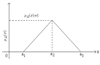
Example 1:In particular ifAe = (a1, a2, a3)be a Triangular
Fuzzy Number (TFN)( cf. Fig. 1) thenµ e
A(x)is defined as
fol-lows
µA˜(x) =
x−a1
a2−a1 fora1≤x < a2
a3−x
a3−a2 fora2< x≤a3
0 otherwise
wherea1, a2anda3are real numbers.
Lemma-1:Let˜a = (a1, a2, a3) )be a triangular fuzzy number
andris a crisp number. The expected value of˜ais
E[˜a] = 1 2
(1−ρ)a1+a2+ρa3
, 0< ρ <1.
= a1+ 2a2+a3
4 , ρ= 0.5. (1)
[image:2.595.325.524.92.221.2]Proof: The Proof of the lemma-1 is in reference in Liu and Liu(2002).
Fig. 1. Triangular Fuzzy Number(TFN)
2.1 Bi-fuzzy set
Generally speaking, a level-2 fuzzy set is a fuzzy set in which the elements are also fuzzy sets, and the bi-fuzzy variable is a fuzzy variable with fuzzy parameters. Level-2 fuzzy sets were origi-nally presented by Zadeh(1971). Such sets are fuzzy sets whose elements themselves are ordinary fuzzy sets. They are very use-ful in circumstances where it is difficult to determine some ele-ments for a fuzzy set.
Definition 1In Mendel (2002), a type-2 fuzzy set, denotedA˜, is characterized by a type-2 membership functionµA˜(x, u), where
x∈Xandu∈J)x⊆[0,1], i.e.,
˜
V ={V , µ˜ V˜( ˜V))| ∀x∈Γ(˜ U) :µV˜ >0} (2)
where each ordinary fuzzy setV˜ is defined by
˜
V ={(x, µV˜(x))| ∀x∈U :µV˜ >0} (3)
For convenience, the membership gradesµV˜( ˜V) of the fuzzy
sets .V˜ ∈ Γ(˜ U) are called ’outer-layer’ membership grades, whereas the membership gradesµV˜(˜x)of the elementsx∈U
are called inner-layermembership grades. Since level-2 fuzzy sets are still fuzzy sets, their mathematical behavior is defined by the fuzzy set operators. Type-2 fuzzy sets were introduced by Zadeh( 1975) as another extension of the concept of an or-dinary fuzzy set, and it was elaborated by Mendel(2002). Such sets are fuzzy sets whose membership grades them as ordinary fuzzy sets. They are very useful in circumstances where it is difficult to determine an exact membership function for a fuzzy set.Normally speaking, a Fu-Fu variable is a fuzzy variable un-der fuzzy environment.
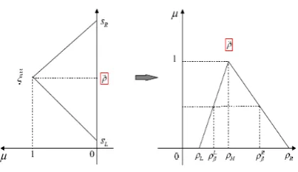
Example 2:˜˜ξ = (sL,ξ, sR˜ )withρ = (ρL, ρM, ρR)is called Fu-Fu variable,( cf. Fig. 2), if the outer-layer and inner-layer membership functions are as follows
µ˜ξ˜(x) =
x−sL ˜ ρ−sL
ifsL≤x≤ρ˜
0 otherwise
sR−x sR−ρ˜
ifρ˜≤x≤sR
and
µρ˜(x) =
x0−ρL ρM−ρL
ifρL≤x0≤ρM
0 otherwise
ρR−x0 ρR−ρM
ifρM≤x0 ≤ρR
whereρ˜is the center ofξ˜, which is a triangular fuzzy variable,
Fig. 2. Triangular Bi-fuzzy variable
Lemma-2:The expected value for the bi-fuzzy variable˜˜c= (˜c− l1,˜c,˜c+r1)withc˜= (c−l2, c, c+r2)we obtain that
E[˜c˜] =c+(r1+r2)−(l1+l2)
4 (4)
Proof:Let˜c˜= (˜c−l1,˜c,˜c+r1), wherec˜= (c−l2, c, c+r2).
Therefore
E(˜˜c) = E(˜c−l1) + 2E(˜c) +E(˜c+r1)
4 (UsingLamma−1)
= E(˜c)−l1+ 2E(˜c) +E(˜c) +r1 4
= 4E(˜c)−l1+r1 4
= E(˜c) +r1−l1 4
= c+r2−l2 4 +
r1−l1 4
= c+(r1+r2)−(l1+l2) 4
Particular case:Whenl2 = 0 = r2 ⇒ c˜˜= ˜c ⇒ E(˜˜c) =
c+r1−l1
4
Lemma-3:Assume thatξ andη are fuzzy/ bi-fuzzy variables with finite expected values. Then for any real numbers a and b, we have
E[aξ+bη] = aE[ξ] +bE[η] (5)
Proof: The proof of the Lemma-3 is in reference Xu and Zhou (2009).
3. ASSUMPTIONS AND NOTATIONS
The model under consideration is developed with the following assumptions and notations.
3.1 Assumptions:
For the product recycling, disposal model, it is assumed that, (i) demand rate is known and time dependent, (ii) shortages are not allowed,
(iii) production rate is time dependent and unknown taken as decision variable ,
(iv) this is a single item inventory model with finite time length, (v) recycling item is same to a new product, it’s rate is constant
and unknown taken as decision variable. (vi) disposal item is rejected unit, it’s rate is constant
and unknown taken as decision variable . (vii) lead time is zero,
(viii) all return units have the same level of quality, (ix) holding cost of non-serviceable item is
less than that for serviceable product. (x) holding cost of non-serviceable item is less
than that for serviceable product.
(xi) Unit production cost is less than the unit recycling cost. (xii) environment pollution cost for production in
industry is also included.
(xiii) The holding costs, setup costs and idle costs are taken to be fuzzy in nature.
(xiv) The unit production cost is taken to be bi-fuzzy in nature.
3.2 Notations:
xSi(t) serviceable stock at time t forithproduction cycle. xSj(t) serviceable stock units at time t forjth
production and recycling cycle.
xR(t) stock of non serviceable units at time t for production cycles.
xRj(t) stock of non serviceable at time t forjth
production and recycling cycle.
u(t) u0+u1t, production rate(decision variable) for
each production up to m cycles.
p(t) p0, constant recycling rate taken as a decision variable.
u0(t) u00+u01t, production rate (decision variable) for each production from m+1 cycle to m+n cycle.
d(t) d0−d1e−βt, demand function,
whered0p, d1pare known andβ >0. (α0+α1t)d(t)return function.
z(t) (z0+z1t), disposal rate(decision variable).
Cp recycling cost per unit. ˜˜
Cu Cu˜˜ 0+ ˜˜
Cu1
u(t)+Cu˜˜ 2(u(t))
γ1+Cu˜˜
3(u(t))γ2,
bi-fuzzy production cost per unit. WhereC˜˜u0is bi-fuzzy raw material cost,
˜˜
Cu1is bi-fuzzy labour cost, ˜˜
Cu2is bi-fuzzy wear and tear cost, ˜˜
Cu3is bi-fuzzy environmental pollution cost
andγi, i= 1,2are positive constants.
Cr purchasing cost per recovered item.
Cz disposal cost per unit item. ˜
˜
hS fuzzy holding cost of serviceable product per unit per unit time.
˜
su fuzzy setup cost for the firstithproduction cycle. ˜
sp fuzzy setup cost for the firstjthrecycling cycle. m number of only production cycles, positive integer.
n number of production and recycling cycles, positive integer.
tu time interval of each production cycle.
tp time interval of each production and recycling cycle.
t0ui time duration of production forithproduction cycle. t0pj time duration of production for
jthproduction and recycling cycle. ˜
Idu fuzzy idle cost for each production cycle.
˜
[image:4.595.311.547.449.787.2]Idp fuzzy idle cost for each recycle cycle.
Fig. 3. Block diagram for production, recycling and disposal model
4. RECYCLING MODEL FORMULATION IN
FUZZY AND BI-FUZZY ENVIRONMENTS
This paper develops a single plant production, recycling-disposal system over a finite time horizon in fuzzy and bi-fuzzy environments. The holding costs, setup costs, idle costs are fuzzy in nature. But the production cost is bi-fuzzy in nature as the purchasing of raw materials faces is how to make purchasing decisions, in order to obtain required raw materials at a lower price and at the same time meet production demand in terms of item, quality, quantity, due date, and so on.
The production and the recycling process are performed in a plant which is located very near to the market and the prod-ucts of plants are continuously transfer to the market. Here, the dynamic demand is satisfied by production and recycling. The used units are bought back and then either recycled or disposed in the said plant. The use units are collected continuously from the customers. Recycling products can be used as new products which are sold again. The rate of production, recycling and dis-posal are assumed to be function of time. The setup cost, idle cost and environment pollution cost for production in industry are also included. The production cost has three parts. (i) raw material cost which is constant per unit product (ii) Labour cost which is inversely proportional per unit product (iii) Environ-mental pollution cost is proportional to the product. The cost is expenditure due to growing environmental concern and accord-ing to the rule of environmental regulations like ’Kyoto Protocol’ for Industry. At the beginning, production satisfies the demand. After sometime, production and recycling fill up the demand. The first m cycles are presented for production and next n cy-cles exist both for production and recycling. The period of each of first m cycle and last n cycle aretuandtprespectively. The
time interval of each of first m cycles is equal. Similarly the time interval of each of last n cycles is equal. Production takest0ui
duration inith, i= 1,2..., mproduction cycle. Also production
and recycling takest0pj duration injth, j = 1,2, ..., n
produc-tion and recycling cycle. We collect reused product at the rate of(α0+α1t)d(t)continuously from the market. At the time of
collection we also consider the disposal at the rate of(z0+z1t).
The total time horizonT =mtu+ntp. The optimization
prob-lem is to maximize total profit over the finite planning horizon, T and it is given in fig-3.
In plant-I, the bi-fuzzy cost functionJ˜˜1is given below:
M inJ˜˜1 = bi-fuzzy production costs + fuzzy holding costs for + serviceable stocks fuzzy set up costs + fuzzy idle costs
= m X
i=1
(i−1)tu+t
0
ui
Z
(i−1)tu
˜˜
Cuu(t)dt+ m X
i=1
itu
Z
(i−1)tu
˜
hSxSi(t)dt
+ mSu˜ + m X
i=1
(tu−t0ui) ˜Idu
+ n X
j=1
mtu+(j−1)tp+t0pj Z
mtu+(j−1)tp
˜˜ Cuu0(t)
+ n X
j=1
mtu+jtp
Z
mtu+(j−1)tp
˜
hSxSj(t)dt
+ nSp˜ + n X
j=1
(tp−t0pj) ˜Idp (6)
In plant-II, the bi-fuzzy cost functionJ˜˜2is given below:
M inJ˜˜2 = fuzzy holding costs for NS stocks
+ fuzzy recycling stock + collect cost + disposal cost
= m X
i=1
itu
Z
(i−1)tu
˜
hRxRi(t)}dt
+ n X
j=1
mtu+jtp
Z
mtu+(j−1)tp
˜
hRxRj(t)dt
+ n X
j=1
mtu+(j−1)tp+t
0
pj
Z
mtu+(j−1)tp
Cpp(t)dt
+ T Z
0
Cr(α0+α1t)d(t) +Czz(t)
dt (7)
subject to
dxSi(t) dt =
(u(t)−d(t)
if(i−1)tu≤t≤(i−1)tu+t0ui
−d(t) if(i−1)tu+t0ui≤t≤itu
(8)
dxSj(t) dt =
u0(t) +p(t)−d(t)
ifmtu+ (j−1)tp≤t≤mtu +(j−1)tp+t
0
pj −d(t)
ifmtu+ (j−1)tp+t0pj≤t≤mtu+jtp
dxR(t) dt =
(α0+α1t)d(t)−z(t)if0≤t≤mtu (10)
dxRj(t) dt =
(α0+α1t)d(t)−p(t)−z(t)
ifmtu+ (j−1)tp≤t≤mtu +(j−1)tp+t0pj
(α0+α1t)d(t)−z(t)
ifmtu+ (j−1)tp+t
0
pj≤t≤mtu+jtp
(11)
where
d(t) = d0−d1e
−βtx
S(0) = 0 =xS(itu), xS(jtp) = 0 xR(0) = 0, u(t) =u0+u1t, p(t) =p0, z(t) =z0+z1t
u0(t) = u00+u01t i= 1,2, ..., m, j= 1,2, ..., n.
Where the bi-fuzzy variables are given by Cui˜˜ = ( ˜Cui − Cui1,Cui,˜ Cui˜ + Cui3), with Cui˜ = (Cui −
Cui2, Cui, Cui+Cui4), i= 1,2,3.
And the TFNs are given by
˜
hi = (hi1, hi2, hi3), i=R, S, ˜
Idj = (Idj1, Idj2, Idj3), j=u, p.
5. EQUIVALENT CRISP MODEL
In plant-I, the expected cost functionE[J˜˜1]is given below:
M in E[J˜˜1] =
m X
i=1
(i−1)tu+t0ui Z
(i−1)tu
E[C˜˜u]u(t)dt
+ m X i=1 itu Z
(i−1)tu
E[˜hS]xSi(t)dt+ m X
i=1
(tu−t0ui)E[ ˜Idu]
+ mE[ ˜Su] + n X
j=1
mtu+(j−1)tp+t0pj Z
mtu+(j−1)tp
E[Cu˜˜ ]u0(t)
+ n X
j=1
mtu+jtp
Z
mtu+(j−1)tp
E[˜hS]xSj(t)dt
+ nE[ ˜Sp] + n X
j=1
(tp−t0pj)E[ ˜Idp] (by lemma-3) (12)
In plant-II, the expected cost functionE[J˜˜2](by using lemma-3)
is given below:
M inE[J˜˜2] =
m X
i=1
itu
Z
(i−1)tu
E[˜hR]xRi(t)}dt
+ n X
j=1
mtu+jtp
Z
mtu+(j−1)tp
E[˜hR]xRj(t)dt
+ n X
j=1
mtu+(j−1)tp+t0pj Z
mtu(j−1)tp
Cpp(t)dt
+ T Z
0
Cr(α0+α1t)d(t) +Czz(t)
dt(13)
Subject to (8)-(11).
6. SOLUTION METHODOLOGY
Using (12)-(14), from (8) the serviceable stock function for
ith(i= 1,2, ..., m)production cycle is given by
xSi(t) =
(u0−d0)(t−(i−1)tu) +u1
t2−((i−1)t
u)2
2 −d1
(e−βt−e−β(i−1)tu)
β
if(i−1)tu≤t≤(i−1)tu+t0ui xSi((i−1)tu+t
0
ui)−d0(t−(i−1)tu−t
0
ui) −d1
(e−βt−e−β((i−1)tu+t0ui)
)
β
if(i−1)tu+t0ui≤t≤itu
and using (12)-(14), from (9) the serviceable stock function for
jth(j= 1,2, ..., n)production and recycling cycle is given by
xSj(t) =
(u00+p0−d0)(t−mtu−(j−1)tp) +u01t2−(mtu+(j−1)tp)2
2
−d1
(e−βt−e−β(mtu+(j−1)tp))
β
ifmtu+ (j−1)tp≤t≤mtu
+(j−1)tp+t0pjxSj(mtu+ (j−1)tp) −d0(t−mtu−(j−1)tp−t
0
pj) −d1
(e−βt−e−β(mtu+(j−1)tp+t
0
pj)) β
ifmtu+ (j−1)tp+t0pj≤t≤mtu+jtp
(14)
Again using (12)-(14), from (10) non serviceable stock only pro-duction cycles is given by
xR(t) =
(α0d0−z0)t+ (α1d0−z1)t
2
2 −α0d1 (1−e−βt)
β +α1d1
te−βt β −α1d1
(1−e−βt)
β2 if0≤t≤mtu
(15)
and also using (12)-(14), from (11) the non serviceable stock for
jth(j= 1,2, ..., n)production and recycling cycle is given by
xRj(t) =
xR(mtu+ (j−1)tp) + (α0d0−p0−z0) (t−mtu−(j−1)tp)
+(α1d0−z1)
t2−(mt
u+(j−1)tp)2
2 −α0d1
(e−β(mtu+(j−1)tp)−e−βt) β
+α1d1
(te−βt−(mt
u+ (j−1)tp)e−β(mtu+(j−1)tp)) β
−α1d1
(e−β(mtu+(j−1)tp)−e−βt) β2
ifmtu+ (j−1)tp≤t≤mtu+ (j−1)tp+t0pj xRj(mtu+ (j−1)tp+t0pj) + (α0d0−z0) (t−mtu−(j−1)tp−t
0
pj) +(α1d0−z1)
t2−(mtu+ (j−1)tp+t0
pj)2 2
−α0d1(e
−β(mtu+(j−1)tp+t0 pj)−e−βt)
β
+α1d1(te−βt−(mtu+ (j−1)tp+t
0
pj) e−β(mtu+(j−1)tp+t0pj)
)1
β −α1d1
(e−β(mtu+(j−1)tp+t0pj) −e−βt) β2
ifmtu+ (j−1)tp+t0pj≤t≤mtu+jtp
In plant-I, the expected cost functionE[J˜˜1]is given below:
E[J˜˜1] =
m X
i=1
E[C˜˜u0]
u0t
0
ui+ u1
2
((i−1)tu+tui)2
− ((i−1)tu)2
+E[Cu˜˜ 1]t
0
ui (17)
+ E[Cu˜˜ 2] u1(γ1+ 1)
(u0+u1(i−1)tu+t
0
ui) γ1+1
− (u0+u1(i−1)tu+t
0
ui) γ1+1
+ E[ ˜˜ Cu2]
u1(γ2+ 1)
(u0+u1(i−1)tu+t
0
ui) γ2+1
− (u0+u1(i−1)tu+t
0
ui) γ2+1
+ (18)
E[˜hS]((u0−d0)(
((i−1)tu+t0ui)2−((i−1)tu)2 2
+ u1 2 (
((i−1)tu+t0ui)3−((i−1)tu)3 3
−((i−1)tu)2t0ui) + m X
i=1
(tu−t0ui)E[ ˜Idu]
+ d1
(e−β((i−1)tu+tui0 )−e−β(i−1)tu) β2
+d1
e−β(i−1)tut0 ui
β +xSi((i−1)tu+t
0
ui)(tu−t
0
ui)
− d0
(itu)2−((i−1)tu+t0
ui)2 2
+d0
(i−1)tu+t0ui)(tu−t
0
ui) + n X
j=1
(tp−t0pj)E[ ˜Idp]
+ d1
(e−β(itu)−e−β((i−1)tu+t0ui))
β2
+ d1
e−β((i−1)tu+t
0
ui)(tu−t0 ui)
β +mE[˜su] +nE[˜sp]
+ n X
j=1
E[Cu˜˜ 0]
u00t0pj+u
0
1 2
(tu+ (j−1)tp+t0pj)2
− (mtu+ (j−1)tp)2
+E[Cu˜˜ 1]t
0
pj
+ E[ ˜˜ Cu2]
u1(γ+ 1)
u00+u
0
1(tu+ (j−1)tp+t
0
pj γ+1
−
u00+u01mtp+ (j−1)tu+t0pj γ+1
+ E[˜hS]((u00+p0−d0)(
(mtu+ (j−1)tp+t0pj)2 2
− (mtu+ (j−1)tp)t0pj) + u01
2(
(mtu+ (j−1)tp+t0pj)3 3
− ((mtu+ (j−1)tp)2t0
pj) +d1
(e−β(mtu+(j−1)tp+t
0
pj)) β2
+ d1
e−β(mtu+(j−1)tp)t0
pj
β +xSj(mtu+ (j−1)tp+t
0
pj)
− d0
(mtu+jtp)2−(mtu+ (j−1)tp+t0
pj)2 2
+ d0(mtu+ (j−1)tp+t
0
pj)(tp−t
0
pj)
+ d1
(e−β(mtu+jtp)−e−β(mtu+(j−1)tp+t0pj) ) β2
+ d1
e−β(mtu+(j−1)tp+t0pj)
(tp−t0pj)
β )
In plant-II, the expected cost functionE[J˜˜2]is given below:
M in E[J˜˜2] =E[˜hR]
(α0d0−z0) (mtu)2
2
+ (α1d0−z1) (mtu)3
6 − α0d1
β (mtu−
1−e−βmtu β )
+ E[˜hR] n X
j=1
[xRj(mtu+ (j−1)tp)t0pj+ (α0d0−p0
−z0)(
(mtu+ (j−1)tp+t0pj)2−(mtu+ (j−1)tp)2 2
− (mtu+ (j−1)tp)tpj0 ) + ((α1d0−z1) 2
((mtu+ (j−1)tp+t
0
pj)3−(mtu+ (j−1)tp)3 3
− (mtu+ (j−1)tp)2t0pj)
− α0d1β−2(e
−β(mtu+(j−1)tp+t0pj)
−e−β(mtu+(j−1)tp))
− α0d1
e−β(mtu+(j−1)tp)t0
pj β
− α1d1
(mtu+ (j−1)tp)e−β(mtu+(j−1)tp)
β t
0
pj
− α1d1((mtu+jtp)e−β(mtu+jtp) −(mtu+ (j−1)tp+t0pj)e
−β(mtu+(j−1)tp+t0pj) )
− α1d1
e−β(mtu+(j−1)tp)t0 pj β2
−α1d1(e
−β(mtu+(j−1)tp+t0pj)
−e−β(mtu+(j−1)tp))
+ xRj(mtu+ (j−1)tp+t0pj)(tp−t0pj)
−(α0d0−z0)(
(mtu+jtp)2−(mtu+ (j−1)tp+t
0
pj)2 2
− (mtu+ (j−1)tp+t0pj)(tp−t0pj))
−(α1d0−z1) 2 (
(mtu+jtp)3−(mtu+ (j−1)tp+t0
pj)3 3
− (mtu+ (j−1)tp+t
0
pj)
2(t
p−t
0
pj)) −α0d1(e−β(mtu+jtp)−e
−β(mtu+(j−1)tp+t0pj) )
− α0d1e
−β(mtu+(j−1)tp+t
0
pj)(tp−t0 pj)
−α1d1
(mtu+ (j−1)tp+t0pj)e−β(mtu+(j−1)tp+t
0
pj)
β (tp−t
0
pj) − α1d1β−2((mtu+jtp)e−β(mtu+jtp)
−(mtu+ (j−1)tp+t0pj)e
−β(mtu+(j−1)tp+t0pj) )
− α1d1
(e−β(mtu+jtp)−e−β(mtu+(j−1)tp+t
0
−α1d1
e−β(mtu+(j−1)tp+t0pj) (tp−t
0
pj)
β2 +spj
b2]
+ Cs(d0T−d1
1−e−βT β )
−Cr
α0d0T+
α1d0T2 2 −
α0d1(1−e−βT)
β
+ α1d1T e
−βT
β −
α1d1(1−e−βT)
β2
−Cz(z0T+
z1T2 2 )
+ n X
j=1
Cptp
Where (By using Lemma-1)
E[˜hj] = (hR1+ 2hR2+hR3)
4 , j=R, S
E[ ˜Idk] = (Idk1+ 2Idk2+Idk3)
4 , k=u, p
E[ ˜Sk] = (Sk1+ 2Sj2+Sk3)
4 , k=u, p
and (By using Lemma-2)
E[Cui˜˜ ] = Cui+(Cui2+Cui4)−(Cui1+Cui3)
4 , i= 0,1,2
E[C˜˜
0
ui] = C
0
ui+
(Cui0 2+Cui0 4)−(Cui0 1+Cu003)
4 , i= 0,1,2
The total expected cost function is given by
MaxJ= E[J˜˜1] +E[J˜˜2] (19)
and (8) -(14) (20)
The objective function (23) with constraints (24) is minimized using the following GA optimization technique.
7. GENETIC ALGORITHM(GA) FOR
SINGLE-OBJECTIVE PROGRAMMING PROBLEM
Genetic Algorithms are exhaustive search algorithms based on the mechanics of natural selection and genesis (crossover, mutation etc.) and have been developed by Holland (cf. Holland (1975)), his colleagues and his students at the University of Michigan (cf. Goldberg (1989)).
A GA for a particular problem must have the following six com-ponents.
(a) A genetic representation for potential solu-tions(chromosomes) to the problem
(b) A way to create aninitial populationof potential solutions (chromosomes).
(c) A way toevaluate fitnessof each solution.
(d) An evolution function that plays the role of environment, rat-ing solutions in term of their fitness, i.e.,selection processfor mating pool.
(e) Genetic operators-crossover,mutationthat alter the compo-sition of children
(f) Values of different parameters that the genetic algorithm uses (Population size, probabilities of applying genetic opera-tors etc).
Procedures for different GA components
(a) Chromosome representation:The concept of chromosome is normally used in the GA to stand for a feasible solution to the problem. A chromosome has the form of a string of genes that
can take on some value from a specified search space. The spe-cific chromosome representation varies based on the particular problem properties and requirements. Normally, there are two types of chromosome representation – (i) the binary vector rep-resentation based on bits and (ii) the real number reprep-resentation. In this research work, the real number representation scheme is used.
Here, a ’K dimensional real vector’ X=(x1, x2, .... xK) is used
to represent a solution, where x1, x2, .... xKrepresent different
decision variables of the problem.
(b) Initialization:A set of solutions (chromosomes) is called a population. N such solutions X1, X2, X3, ... XN are randomly
generated from search space by random number generator such that each Xisatisfies the constraints of the problem. This
solu-tion set is taken as initial populasolu-tion and is the starting point for a GA to evolve to desired solutions. At this step, probability of crossoverpcand probability of mutationpmare also initialized. These two parameters are used to select chromosomes from mat-ing pool for genetic operations- crossover and mutation respec-tively.
(c) Fitness value:All the chromosomes in the population are evaluated using a fitness function. This fitness value is a mea-sure of whether the chromosome is suited for the environment under consideration. Chromosomes with higher fitness will re-ceive larger probabilities of inheritance in subsequent genera-tions, while chromosomes with low fitness will more likely be eliminated. The selection of a good and accurate fitness function is thus a key to the success of solving any problem quickly. In this thesis, value of a objective function due to the solution X, is taken as fitness of X. Let it be f(X).
(d)Selection process to create mating pool:Selection in the GA is a scheme used to select some solutions from the popula-tion for mating pool. From this mating pool, pairs of individu-als in the current generation are selected as parents to reproduce offspring. There are several selection schemes, such as roulette wheel selection, local selection, truncation selection, tournament selection, etc. Here, roulette wheel selection process is used in different cases. This process consists of following
steps-(i) Find total fitness of the population F=
N P i=1
f(Xi)
(ii) Calculate the probability of selection priof each solution Xi
by the formula pri=f(Xi)/F .
(iii) Calculate the cumulative probability qri for each solution
Xiby the formula qri= i P j=0
prj
(iv) Generate a random number ’r’ from the range [0..1]. (v) If r<qr1 then select X1otherwise select Xi(2≤i≤N) where
qri−1≤r<qri.
(vi) Repeat step (iv) and (v) N times to select N solutions from current population. Clearly one solution may be selected more than once.
(vii) Let us denote this selected solution set byP1(T).
(e)Crossover: Crossover is a key operator in the GA and is used to exchange the main characteristics of parent individuals and pass them on the children. It consists of two steps:
(i) Selection for crossover: For each solution ofP1(T)generate
a random number r from the range [0..1]. If r<pc then the
solution is taken for crossover, where pcis the probability of
crossover.
(ii) Crossover process: Crossover taken place on the selected solutions. For each pair of coupled solutions Y1, Y2 a
ran-dom number c is generated from the range [0..1] and Y1,
where Y11=cY1+(1-c)Y2 , Y21=cY2+(1-c)Y1, providedY11,
Y21satisfied the constraints of the problem.
(f) Mutation: The mutation operation is needed after the crossover operation to maintain population diversity and recover possible loss of some good characteristics. It is also consist of two steps:
(i) Selection for mutation: For each solution ofP1(T)generate
a random number r from the range [0..1]. If r< pmthen the solution is taken for mutation, where pmis the probability of
mutation.
(ii) Mutation process: To mutate a solution X=(x1, x2, ., xK)
select a random integer r in the range [1..K]. Then replace xr by randomly generated value within the boundary of rth
component of X.
Following selection, crossover and mutation, the new population is ready for it’s next iteration, i.e.,P1(T)is taken as population
of new generation. With these genetic operations a simple ge-netic algorithm takes the following form. In the algorithm T is iteration counter, P(T) is the population of potential solutions for iteration T, Evaluate(P(T)) evaluate fitness of each members of P(T).
GA Algorithm
1. Set iteration counter T=0.
2. Initialize probability of crossover pcand probability of
muta-tion pm.
3. Initialize P(T). 4. Evaluate(P(T)). 5. Repeat
a. Select N solutions from P(T), for mating pool using Roulette-wheel selection process. Let this set beP(T)1.
b. Select solutions fromP(T)1, for crossover depending on
pc.
c. Made crossover on selected solutions for crossover to get populationP(T)2.
d. Select solutions fromP(T)2, for mutation depending on
pm.
e. Made mutation on selected solutions for mutation to get populationP(T+ 1).
f. T←T+ 1.
g. EvaluateP(T).
6. Until(Termination condition does not hold). 7. Output: Fittest solution(chromosome) of P(T).
8. NUMERICAL EXPERIMENT
To illustrate the production-recycling model numerically, we consider input data in Tables-1,-2 & -3 for crisp data, fuzzy data and bi-fuzzy data respectively. For these input data and by using the above single objective genetic algorithm technique§7and using Lemma-2, we solve the problem (23)-(24) and we obtained the optimal productions, optimal recycling and optimal disposal which areu(t) = 25.19 + 0.6t, u0(t) = 17.2 + 0.4t, p(t) = 11
and z(t) = 0.71 + 0.16t. Also the optimal values of
xSi(t), xSj(t), xR(t), u(t), u0(t), d(t)andp(t)are evaluated using (23)-(24) for different values of t. We have shown the optimum results of xSi(t), xR(t), u(t) and d(t) of production-cycle in Table-4. Similarly, the optimum results of
xSj(t), xRj(t), u0(t), p(t) and d(t) for the production and recycling-cycle are presented in Table-5. We get optimal profit by using GA technique as871.349$.
Table-1 Input crisp Data:
d0 d1 β Cp Cz
in $ in $
[image:8.595.311.551.96.412.2]15 0.2 0.05 1.6 0.15 Cr γ1 γ2 α0 α1 T 0.11 0.1 0.12 0.12 0.1 15
Table-2
Input fuzzy Data: (in $)
˜
hR hS˜ Idu˜
(1.1,1.3,1.5) (1.3,1.5,1.7) (3,4,5) ˜
Idp Su˜ Sp˜ (2.5,3.5,4.6) (3,4,5) (3,5,5)
Table-3
Input bi-fuzzy Data:(in $)
˜˜
Cu0 Cu˜˜ 1
( ˜Cu0−5,Cu˜ 0,Cu˜ 0+ 7) ( ˜Cu1−14,Cu˜ 1,Cu˜ 1+ 15) ˜
Cu0= (3.5,6.0,7.5) C˜u1= (11.5,15.6,20.8) ˜˜
Cu2 Cu˜˜ 3
( ˜Cu2−1,Cu˜ 2,Cu˜ 2+ 2) ( ˜Cu3−0.9,Cu˜ 3,Cu˜ 3+ 1.4) ˜
Cu2= (1.4,1.7,2.9) C˜u3= (0.6,1,2.1)
Table-4
Optimal values of xSj(t), xRj(t), u0(t), p(t) and d(t),
j= 1,2,3.
t 0 1.28 3 3.01 4.01 6 xSi(t) 0 15.33 0 0.16 16.2 0 xR(t) 0 1.73 6.78 6.86 8.28 15.4
[image:8.595.316.554.442.662.2]u(t) 29.13 29.77 − 30.53 31.14 − d(t) 15.7 15.32 16.63 15.67 15.42 14.97
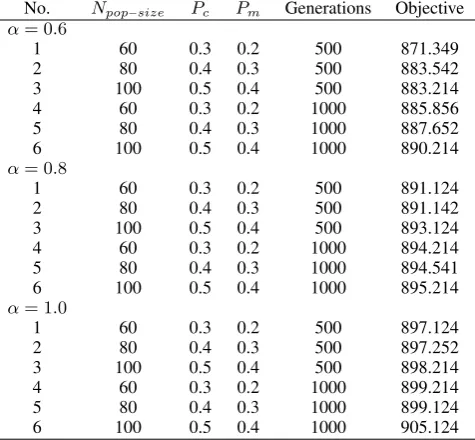
Table-5
Comparison of the results obtained with different GA parame-ters.
No. Npop−size Pc Pm Generations Objective α= 0.6
1 60 0.3 0.2 500 871.349
2 80 0.4 0.3 500 883.542
3 100 0.5 0.4 500 883.214
4 60 0.3 0.2 1000 885.856
5 80 0.4 0.3 1000 887.652
6 100 0.5 0.4 1000 890.214
α= 0.8
1 60 0.3 0.2 500 891.124
2 80 0.4 0.3 500 891.142
3 100 0.5 0.4 500 893.124
4 60 0.3 0.2 1000 894.214
5 80 0.4 0.3 1000 894.541
6 100 0.5 0.4 1000 895.214
α= 1.0
1 60 0.3 0.2 500 897.124
2 80 0.4 0.3 500 897.252
3 100 0.5 0.4 500 898.214
4 60 0.3 0.2 1000 899.214
5 80 0.4 0.3 1000 899.124
6 100 0.5 0.4 1000 905.124
Table-5 shows the experimental results obtained by a GA with different GA parameters. The tested GA parameters contain the population sizeNpop−size, the probability of crossoverP cand
repre-sents the optimum result for non serviceable stock. The increas-ing demand rate is very small.
Fig. 4. Optimal production, demand, recycling and serviceable stock
9. CONCLUSION
In this paper, we develop a two plants production, recycling-disposal system over a finite time horizon in fuzzy and bi-fuzzy environment. The holding cost, setup cost, idle cost are fuzzy in nature. But the production cost is bi-fuzzy in nature as the purchasing of raw materials faces how to make purchasing deci-sions, in order to obtain required raw materials at a lower price and at the same time meet production demand in terms of item, quality, quantity, due date, and so on. Here, the dynamic demand is satisfied by production and recycling. Recycling products can be used as new products which are sold again. The rate of pro-duction, recycling and disposal are assumed to be control vari-ables. The cost is expenditure due to growing environmental con-cern and according to the rule of environmental regulations like ’Kyoto Protocol’ for Industry. At the beginning, production sat-isfies the demand. After sometime, production and recycling fill up the demand. The total cost is minimized as an optimal control problem. It is solved by single objective genetic algorithm tech-nique. The model is illustrated through numerical examples and results are also presented both in tabular form only. The model can be extended for imperfect production, recycling-disposal op-timization problem in uncertain environment.
10. REFERENCES
[1] Dobos, I. and Richter, K., (2000). A production / recycling model with quality consideration. International Journal of Production Economics, 104, 571-579.
[2] Giri, B. C., Yun, W. Y and Dohi, T., (2005). Optimal de-sign of unreliable productioninventory systems with variable production rate, European Journal of Operational Research, 162: 372 386.
[3] Gold Goldberg,D., (1989). Genetic Algorithems in Search, Obtimization and Machine Learning, Addision Wealey, MA, USA.
[4] Gottwald, S., (1979). Set theory for fuzzy sets of higher level. Fuzzy Sets and Systems 2(2), 125-151.
[5] Grzegorzewski, P., (2002). Nearest interval approximation of a fuzzy number, Fuzzy Sets and Systems 130, 321-330. [6] Holland, H. J., (1975). Adaptation in Natural and Artificial
Systems, University of Michigan.
[7] Gungor,A., Gupta,S. M., (1999). Issues in environmentally conscious manufacturing and product recovery: a survey, Computers & Industrial Engineering, 36, 811-853.
[8] Ilgin,M. A. , Gupta,S. M., (2010). Environmentally con-scious manufacturing and product recovery (ECMPRO): A review of the state of the art. Journal of Environmental Man-agement 91,(3), 563-591.
[9] Liu, Y., Liu,B., (2003). A class of fuzzy ramdom optimiza-tion: expected value models, Information Science 155, 89-102.
[10] Liu,B., Liu,Y.K., (2002). Expected value of Fuzzy vari-able and Fuzzy expected value Models, IEEE Transactions of Fuzzy Systems 10(4), 445-450.
[11] Mendel, J.M., John, R.I.B., (2002). Type-2 Fuzzy Sets Made Simple. IEEE Transactions on Fuzzy Systems 10(2), 117-127.
[12] Minner, S. and Kleber, R., (2001). Optimal control of pro-duction and remanufacturing in a simple recovery model with linear cost functions, Spektrum, 23: 3-24.
[13] Maiti, M. K., Maiti,M., (2007). Determination of with-drawal schedule in single-species cultivation via genetic algorithm. Applied Mathematics and Computation 188(1), 322-331
[14] Maity, A.K., Maity,K., Maiti,M., (2008). A production-recycling-inventory system with imprecise holding costs, Applied Mathematical Modelling 32, 2241-2253.
[15] Maity, A.K., Maity,K., Mondal.S., Maiti,M., (2009). A Production-recycling-inventory model with learning effect, Optimization and Engineering 10, 427-437.
[16] Maity,K., Maiti,M., (2005). Numerical approach of multi-objective optimal control problem in imprecise environment, Fuzzy Optimization and Decision Making, Netherland, 4(4), 313-330.
[17] Mendel, J.M.,(1999). Computing with words when words can mean different things to different people. Presented at Internat. ICSC Congress on Computational Intelligence: Methods, Applications, 3rd Annual Symp. on Fuzzy Logic and Applications, Rochester, New York, 22-25
[18] Zadeh, L.A.:(1975) The concept of a linguistic variable and its application to approximate reasoning, Information Sci. 8, 199-249.
[19] Taleizadeh, A., Niaki S., Seyedjavadi, S M. H.,(2012) Multi-product multi-chance-constraint stochastic inventory control problem with dynamic demand and partial back-ordering: A harmony search algorithm, Journal of Manufac-turing Systems, 31(2) 204-213.
[20] Marusak, Marusak,P. M., Tatjewski, P., (2009). Effective dualmode fuzzy dmc algorithmswith online quadratic opti-mization and guaranteed stability, Int. J. Appl. Math. Com-put. Sci., Vol. 19, No. 1, 127-141.
[21] Xu, J., Zhou,X., (2009). Fuzzy Link Multiple-Objective Decision Making, Springer- Verlag, Berlin.
[22] Zadeh,L., (1965). Fuzzy sets, Information and Control. 8, 338-353.
[23] Zadeh, L.,(1971). Quantitative fuzzy semantics. Informa-tion Sciences 3(2),177-200.
[24] Zhang, H. C., Kuo, T. C., Lu, H., (1997). Environmentally con-scious design and manufacturing: A state-of-the-art survey, Jour-nal of Manufacturing, 16, 352-371.
11. AUTHOR PROFILE
D. K. Jana
international journals such as JOS, IJOR, OPSEARCH etc.
K. Maity
K. Maity received his PhD degree in Applied Mathematics from Vidyasagar University in 2006. He is a Lecturer in the Depart-ment of Mathematics, Mugberia Gangadhar Mahavidyalaya, Purba Medinipur. His research and development efforts focus on operational research, optimal control theory, fuzzy mathematics and fuzzy logic. He has received the Prof.M.N. Gopalanan Award for best doctorial thesis from ORSI in 2007. He pub-lished many research papers in reputed international journals such as EJOR,MCM, FODM, AJMMS, Information Sciences,
etc.
T. K. Roy