Analysis of Network Lifetime for Wireless Sensor
Network
Swarup Kumar Mitra
Department of ECE, MCKV Institute of Engineering,
Howrah, India.
Mrinal Kanti Naskar
Jadavpur University
Kolkata-700032
India
Pradipta Ghosh
Jadavpur University Kolkata-700032
India
ABSTRACT
Wireless Sensor Network (WSN) consists of motes which are equipped with limited battery and requires energy management for enhanced Network Lifetime. In this paper we have adopted a deployment strategy which is performed over a region of interest (ROI) obtained from contour integration of one hop to other. The selection of motes depending on the type of application is also analyzed. The necessity of proper resource utilization in a sensor network enables us to propose a realistic radio model which considers the sorted power level from discrete radio model. The utility of Network coding is also adapted for enhanced throughput and robustness of the network.
Keywords
Contour Integration, Event generation model, Packet generation rate, Realistic radio model, Poisson distribution, Network Simulator 2.33.
1.
INTRODUCTION
Wireless Sensor Networks (WSNs) are ad-hoc networks, consisting of spatially distributed devices (motes) using sensor nodes to cooperatively monitor physical or environmental conditions at different locations. Devices in a WSN are resource constrained; they have low processing speed, storage capacity, and communication bandwidth.
Nodes sense the surrounding environmental information and send their report toward a processing center that is called “sink” or base station (BS), where the data will be made available to the user. Such networks have a wide range of potential applications, from military surveillance to habitat monitoring. Hence, it is well accepted that one of the key challenges in unlocking the potential of such wireless sensor networks is estimating the network lifetime so as to see what factors dominate the lifetime and consequently where engineering effort should be invested in each individual deployment scenario. In most settings, the network must operate for long periods of time, but the nodes are battery powered, so the available energy resources limit their overall operation. To minimize energy consumption, most of the device components, including the radio, should be switched off most of the time [7].
Network lifetime is the time duration from the instant of node deployment up to the instant when the network is considered nonfunctional. When a network should be considered nonfunctional is, however, application-specific. It can be, for
they propose a method to assign the number of nodes within each bin in order to maximize the network lifetime
Another important characteristic is that sensor nodes have significant processing capability in the ensemble, but not individually. Nodes have to organize themselves, administering and managing the network all together, and it is much harder than controlling individual devices. Furthermore, changes in the physical environment where a network is deployed make also nodes experience wide variations in connectivity and it influences the networking protocols. The main factors that complicate the design for WSNs can be summarized in:
(i) Fault tolerance: the necessity to sustain sensor networks functionalities without any interruption, after a node failure.
(ii) Scalability: the possibility to enlarge or reduce the network and exact placement of BS.
(iii) Deployment: given a certain environment it should be possible to find the suitable deploying location for each sensor.
(iv) Energy management: the network lifetime needs to be maximized using data handover.
(v) Proper selection of radio model.
(vi) Sensing of an event over a region of interest through event generation model
In this paper we propose to estimate the lifetime of a Wireless Sensor Network (WSN) taking into consideration of all the aspects required to design a network such as: node density, selection of motes, data flow using network model, occurrence of events, packet generation. We also considered discrete radio model for practical feasibility and utilization efficiency of the network. The lifetime of a WSN is affected by many factors which include network architecture, network size, sensor node population model, the generation rate of sensing data, initial battery budget available at each sensor, and data communication protocols. Key data communication protocols include those for medium access control, traffic routing, as well as sleep (or duty cycle) management. With such a large number of factors, accurate lifetime estimation of a sensor networks is a complex task. We investigate accurate lifetime estimation of a sensor networks using discrete radio model. We assume that network sensors are organized into annular rings. Node density is uniform throughout the region of interest (ROI)=ρ. The sink is remotely located inside the ROI and has the capability of communicating to the distant BS.
Hop to hop data flow is estimated for the amount of packet transmitted and amount of packet received where total number of redundant packets also is being considered. Further we derive an event generation model to predict the overall network lifetime. Discrete radio model enables us to derive the flow of data (packets) and transmission rate in each of the sensor motes which gives an expectation for the sustainability of the network. Our objective is to formulate an estimation of network lifetime from the following design parameters obtained
Design parameters:
(i) Network Size and deployment of nodes. (ii) Choice of Sensor Motes.
(iii) Selection of Radio Model. (iv) Network Coding for Data Flow. (v) Event Generation Model
2.
NETWORK SIZE AND DEPLOYMENT
OF NODES:
To design a wireless sensor network it should be possible to find suitable location to deploy the sensors. Energy aware algorithms deploys the nodes either manually (i.e. deterministic) or randomly depending on the nature of application.
[image:2.612.330.549.307.491.2]We have considered a sensor network which is constructed by random deployment of sensor nodes over a Region Of Interest (ROI). A typical data gathering tree with active nodes collectively transmits to the next hop through a leader to the sink. Each hop is defined under a annular ring consisting of active and sleep nodes. Active nodes are those which participate in the data gathering process and sleep nodes remain dormant due to low battery. Selection of active nodes depends on highest priority among neighbors to transmit packets. Below in Fig 1 we have demonstrated a topology of sensor nodes and routing of data transmission through wireless links.
Figure 1: Network Model (multi hop)
The network is divided into several hops depending upon the distance from the base station. The Base station is located radically outward towards periphery. Each node in the sink cluster acts as a root of an independent data gathering tree for collecting data from the network and unicast it to the sink node. Thus the number of data gathering trees in Wireless Sensor Network (WSN) depends upon region of interest (ROI). Node density is uniform throughout the ROI. The sink is remotely located inside the ROI and has the capability of communicating to the distant BS. Each hop reflects a data transmission from one ROI(annular ring) to another ROI.
which proves the generality of the topology. Assuming the node density to be uniform throughout. Let us take the Hop- to – Hop Node Ratio, (βi)
c th c th c th c th i hop i f peripheryo hop i f peripheryo hop i f peripheryo hop i f peripheryo ) 1 ( ) ( ) ( ) 1 (
Ratios of areas under (i+1)th hop & ith hop Ai+1= Area in (i+1)th hop , Ai = Area in (i)th hop
Ai+1 / Ai ( Since ρ. is constant )...(1)So approximate number of nodes in the nth hop of a data gathering tree
1 1 1 2 1 n i i n
... (2)The ROI that contains the sink is called the sink region.
Each ROI has one coordinator and some sensors (devices). The data gathering tree coordinates through a coordinator in each hop and finally routes it to the sink. The network lifetime is defined as the time duration before a ROI in the network is first exhausted. Because the nodes that are closer to the sink assume more relay duty, they may be exhausted first. To equalize lifetime among nodes, a technique called population adjustment is used to adjust the number of nodes in each ROI; ROI that are closer to the sink have more sensors with higher budget. We are interested in answering the following question: how long can a sensor network survive when with a specified topology while working to achieve satisfactory quality of service.
.
3.
SELECTION OF MOTES
A node functions as a device which senses and receives data from its neighbor and communicates with it and the base station (BS). The term “mote” was coined by researchers in the Berkeley NEST (now WEBS [1]) and CENS [2] projects) to refer to these sensor nodes. Each sensor node is equipped with a microcontroller, transceiver, memory, power source and one or more sensors, either internal or external to the sensor board. The motes plays two role for the network : - either data-logging, processing (and/or transmitting) sensor information from the environment, or acting as a gateway in the adhoc wireless
network formed by all the sensors to pass data back to a (usually unique) collection point. In this paper, we analyze and compare different parameters required for selection of motes which could sustain enhanced Network Lifetime. These parameters range from physical characteristics such as size, weight and battery life to electrical specifications for the microprocessor and radio transceiver employed in the respective mote architectures. We have classified the components of the motes into general parameters namely processor and memory, communications capabilities, sensor support and power consumption. The following motes will be discussed: -
TelosB/TmoteSky : - Wireless sensor modules developed from research carried out at UC Berkeley and currently available in similar form factors from both Sentilla and CrossBow Technology.Mica2/MicaZ :- second and third generation wireless sensor networking mote family from CrossBow Technology.SHIMMER:- SHIMMER (Sensing Health with Intelligence, Modularity, Mobility, and Experimental Reusability) is a wireless sensor platform designed to support wearableapplications.
Currently available from Real Time Ltd.IRIS: - latest wireless sensor network module from Crossbow Technologies. Includes several improvements over the Mica2 / MicaZ family of products. Improvements include increased transmission range.
Sun SPOT: - the Sun “Small Programmable Object Technology” (SPOT) is a wireless sensor network mote from Sun Microsystems. Unlike many of the other offerings considered
here, both the hardware and software are open-source. EZ430-RF2480/2500: - the EZ430-RF2480 and EZ430-RF2500 wireless networking solutions from Texas Instruments incorporate the MSP430 microprocessor and CC2480/2500 radio transceiver on each board. These kits are the most inexpensive mote solution reviewed in this paper.
Table1: Mote Specification Mote
Platform
TelosB MicaZ/ Mica2
SHIMMER IRIS Sun SPOT EZ430-RF2500 (USB)
EZ430-RF2480 (Batt)
WxLxH 1.26 x 2.58 x 0.26
1.25 x 2.25 x 0.25
0.8x1.75x0.5 1.25 x 2.25 x 0.25
2.5x1.5x1 1.16 x 3.17 x 0.43
1.02 x 3.72 x 0.55 Weight
batt [g]
14.93 15.07 4.87 21.29 33.49 1.80 1.8
Cost US$ 99/ US $139
US$ 99 EUR 199 US$ 115
US$ 750 US$ 99
US$ 49
Processor TI
MSP430F1611 Atmel Atmega 128 L TI MSP430F1611 Atmel Atmega 128 1 Atmel AT91RM9200 TI MSP430F2274 TI MSP430 F2274
The TelosB/Tmote Sky, MicaZ, SHIMMER and Sun Spot motes employ the 802.15.4 [8] compatible CC2420 radio chip from Texas Instruments [9]. The Iris mote also uses an 802.15.4 compatible chip, namely Atmel’s AT86RF230 [10]. These two radios are packet level radios, with a maximum packet length of 127 bytes. The MicaZ mote uses the Texas Instruments CC1000 [11], the EZ430-RF2500 uses the Texas Instruments CC2500 [12] while the EZ430-RF2480 uses the CC2480 [13], once again from Texas Instruments. The CC1000 and CC2500 are both bit level radios and the CC2480 is a Zigbee [14] compatible packet level radio which contains a Zigbee coprocessor. In addition to the CC2420 the SHIMMER also contains a second
radio, a class 2 Bluetooth radio compatible with the Mitsumi
WML-C46 series.
In this paper we analyzed the platform necessary for the motes to function properly under different circumstances.
TinyOS:
TinyOS is an embedded operating system expressly designed for WSNs. The basic concepts behind TinyOS are: application compiled and used for programming a single node.
• Hurry Up and Sleep: Philosophy; so when a node wakes up for an event, it has to execute the associated action as fast as possible, then go back to sleep. Because of the extremely limited resources of the hardware platforms, it is difficult to virtualized system operation to create the kinds of system abstractions that are available in more resource rich systems. The concurrency model and abstractions provided by operating system therefore significantly impact the design and development process. The TinyOS 2.x family is the latest stable branch of the operating sys-
tem and is used in this section to describe the basic design principles. The TinyOS development environment directly supports a variety of device programmers and permits programming each device with a unique address at tribute without having to compile the source code each time. The TinyOS system, libraries and applications are written in nesC, a version of C that was designed for programming embedded systems. The characteristics of TinyOS 2.x are listed as [24]: • Resource constrained concurrency
Concurrency is the main important software challenge. The system manages several components, as sensors, ADCs, radio and flash memory. Generally, an operation is started on a device, which runs concurrently with the main processor until generating a response.
Meanwhile, other devices may also need service, requiring the system to manage several event streams. A conventional OS uses multiple threads, each with its own stack. The thread dedicated to a device issues a command and then sleeps or polls until the operation completes. The OS switches among threads by saving and restoring their registers, and threads coordinate with others by using shared variables as flags and semaphores. This is problematic for embedded designs because multiple stacks must be kept in memory and each thread can potentially interact with any other whenever it accesses a shared variable. This can lead to deadlocks, requiring complex schedulers to meet real-time requirements and deadlines. TinyOS attacks the problem by offering different levels of
concurrency, in a structured event-driven execution.
• Structured event-driven execution: TinyOS provides a structured event-driven model. A complete system configuration is formed by ’wiring’ together a set of components for a target platform and application domain. Components are restricted objects with well-defined interfaces, internal state, and internal concurrency. Primitive components encapsulate hardware elements (radio, ADC, timer, bus ...). Their interface reflects the hardware operations and interrupts; the state and concurrency is that of the physical device. Higher-level components encapsulate software functionality, but with a similar abstraction. They provide commands, signal events, and have internal handlers, task threads, and state variables. This approach accommodates hardware evolution, including major changes in the hardware/software boundary, by component replacements. Its memory footprint is small, despite supporting extensive concurrency, requiring only a single stack and a small task queue. However, the modular construction provides flexibility, robustness, and ease of programming. A restricted form of thread, called a task, is available within each component, but interactions across components are through explicit command/event interfaces. The wiring of components and the higher priority of asynchronous events over tasks permit the use of simple schedulers, and in TinyOS 2.0 even the scheduler is replaceable.
• Components and bidirectional interfaces : TinyOS supports component composition, system-wide analysis, and network data types. A component has a set of bidirectional command and event interfaces implemented either directly or by wiring a collection of subcomponents. The compiler optimizes the entire hierarchical graph, validates that it is free of race conditions and deadlocks, and sizes resources. The TinyOS community has developed plug-ins for integrated solutions and several visual
Table II Radio Chip Specification Radio
Module
Frequency (MHz)
Modulation Data Rate Tx Power (dBm) Rx Sensitivity (dBm)
TI CC1000 300 - 1000 FSK 76.8 kBaud -20 - 10 -110 (at 2.4
kBaud)
TI CC2420 2400 - 2483.5 OQPSK 250 kbps -24 - 0 -95
TI CC2500 2400 - 2483.5 OOK, 2-FSK, GFSK, MSK
500 kBaud -30 - 1 -108 (at 2.4
kBaud)
TI CC2480 2400 - 2483.5 OQPSK 250 kbps -55.8 -0 -92
Atmel AT86RF23 0
2405 - 2480 OQPSK 250 kbps -17 - 3 -101
Mitsumi WML-C46
programming environments for this component-based programming style. Network data types simplify protocol implementation. While network packets have a particular specified format, data representation in a computer program depends on word width and addressing of the host processor, so most protocol code contains machine-dependent bit-twiddling and run-time parsing. Because TinyOS uses network types with a completely specified representation, the compiler provides efficient access to packet fields on embedded nodes, as well as Java and XML methods for packet handling on conventional computers and gateways.
• Split-phase operations : Split-phase operations are a typical use of bidirectional interfaces. TinyOS has a non-preemptive nature and does not support blocking operations. This means that all long-latency operations have to be realized in a split-phase fashion, by separating the operation-request and the signaling of the completion. The client component requests the execution of an operation using command calls which execute a command handler in the server component. The server component signals the completion of the operation by calling an event handler in the client component. In this way, each component involved in the interaction is
responsible for implementing part of the split-phase operation. • Sensing : TinyOS 2.0 provides sensor drivers, which scale from low-rate, low power sampling of environmental factors to high-rate, low-jitter sampling of vibration or acceleration. Drivers handle warm-up, acquisition, arbitration, and interface specifics. Since sensor selection is closely tiedto the application and mechanical design, drivers must be easily configured and tested, rather than dynamically loaded after market.
• Communication and networking : Communications and networking have driven the TinyOS design as available radios and microcontroller interfaces evolved. The communication subsystem has to meet real-time requirements and respond to asynchronous events while other devices and processes are serviced. The TinyOS 2.0 radio component provides a uniform interface to the full capabilities of the radio chip. The link-level component provides rich media access control (MAC) capabilities, including channel activity detection, collision avoidance, data transfer, scheduling, and power management, allowing networking components to optimize for specific protocols. The TinyOS community has developed networking layers targeted at different applications with different techniques for discovery, routing, power reduction, reliability, and congestion control. These networking layers provide higher-level communication services to embedded applications with a TinyOS programming interface. The most widely used services for WSNs are reliable dissemination, aggregate data collection, and directed routing. To collect and aggregate data from the WSN, nodes cooperate in building and maintaining one or more collection trees, rooted at a gateway or data sink. Each node gathers link-quality statistics and routing cost estimates through all kinds of communication, including routing beacons, packet forwarding, and passive traffic monitoring.
• Storage: Nonvolatile storage is used in WSNs for logging, configuration parameters, files, and program images. Several different kinds of Flash memory are used with different interfaces and different protocols. Lower-layer TinyOS components provide a block storage abstraction for various Flash chips and platform configurations, with one or more application level data services provided on this substrate.
4.
SELECTION OF RADIO MODELS
To obtain enhanced network lifetime we need to select radio models from all aspects of communication. In wireless channel the electromagnetic wave propagation can be modeled as falling off as power law function of distance between the transmitter and receiver. If there is no direct line of sight between the transmitter and receiver then electromagnetic wave will bounce of objects and will arrive from different paths at different time. Once deployed, all the nodes are stationary and cannot replace or recharge their limited batteries. But they have the capability of adjusting their transmission power to control the radio
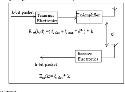
[image:5.612.330.535.198.349.2]coverage
Figure 2: First order radio model
range, such that a node can transmit its k-bit packet directly to the BS (one-hop) or, alternatively, through several intermediate nodes (multi-hop). For wireless communication, the simple first-order radio model, as in figure ? is used to calculate the energy consumption for transmitting and receiving data packets. Let ξelec = 50nJ/bit and ξamp = 100 pJ/bit/m2 [2] denote the
energy consumption rates for operating the electronics in radio transceiver and transmitter amplifier, respectively. We assume ξelec also take into account the energy consumption for
aggregating multiple incoming data packets and generating a single same sized outgoing packet which is known as data fusion. For receiving a k-bit packet, a sensor node consumes Erx
(k) Joule of energy, or,
k
k
E
rx(
)
elec
(1)While for transmitting a k-bit packet to another node over a distance of d meters, the energy consumption is
k
d
d
k
)
(
R
L
I
I
V
P
transmit
remaining
ROON
startup
plevel
(3)
Where,
V
remaining= remaining current voltage of the mote, ROONI
=Current required for radio oscillator to start.startup
=start up time.I
plevel= current at a power level.L=packet size, R= rate of transmission.
)
(
R
L
I
V
E
receive
remaining
R
(4)Energy dissipation for reception or transmission is constant for a particular power level. Initial Energy =Ei
i R
T
R
E
R
E
E
1
2
(5) [image:6.612.85.260.335.485.2]The transmit and receive power level is selected from the Table I and II which provides energy consumed in transmission of 100 byte packet considering the different power levels used by CC24220.We have neglected power level 15 as it has a power output of -7dbm and simulations yields that the distance of operation of this power level is so close to power levels 11 and 19 such that it becomes meaningless to take this power level in the context of number of packets of energy sent in the simulations. The number of packets sent in one transmission is taken to be as 5. So a total of 500 bytes are sent.
Table 3:
Power level (k)
Pout
[dBm] Ix
mA PTX
mW
Etx/ packet
[μJ]
3 -25.00 17.04 30.67 98.14
7 -15.00 15.78 28.40 90.88
11 -10.00 14.63 26.33 84.26
19 -5.00 12.27 22.08 70.66
23 -3.00 10.91 19.62 62.78
27 -1.00 9.71 17.47 55.90
31 0 8.42 15.15 48.48
As most data dissemination algorithms depend upon a centralized base station configuration we will focus upon these types of networks. This network configuration provides some major advantages for discrete power level selection. Firstly, only the base station needs to track and store which nodes can communicate and at which power levels. This frees up memory and storage space, which is limited on each mote, allowing for more data aggregation to occur or storing more data before transmitting it back to the base station. Secondly, with a centralized configuration the base station will know the exact power levels of each mote are using for transmitting and therefore the exact power cost. In order to select the best power levels in a real world deployment we propose that a network initialization period is used. In this period, each mote takes a turn and broadcasts a packet at each power level with the assigned mote id and the transmission power level being used. Each other mote in the network will listen for the packet and track the lowest power that can be used for communication from that mote. Once every mote has participated in the initialization period, they generate a packet containing their mote id and an array of incoming packet information. This incoming packet
information will contain the incoming mote id, lowest received power level and the associated RSSI. This packet is transmitted to the base station for storage and processing, which relieves the mote from storing the information. With this information at the base station, the data dissemination algorithms can be optimized for the exact costs and the base station can dictate which power levels should be used when it broadcasts schedules to motes in the network.
5.
NETWORK CODING
Network Coding is a new area for the researchers to utilize the intermediate motes within a routing path of a sensor network. It produces two outcomes
(i) Potential improvement of throughput. (ii) High degree of robustness.
Network coding is a unique concept in data gathering where instead of forwarding data it recombines several input packets into one or several output packets. This allows a larger degree of flexibility in the technique of packets to be combined. The forwarding of packets simply allows the nodes to repeat but network coding allows the packets to get coded or to combine linearly into an outgoing packet. This doesn’t resemble concatenation but it allows the data to spread over the entire network. It can be applied over one source and one sink to multiple sources and multiple sink networks. The sources are mutually independent.
We have illustrated its information flow over various network as shown below.
S= Source and t =Sink .
A one source and one sink Network.
Assume that we multicast two data bits b1 and b2 from the source node S to both the nodes Y and Z in the acyclic network depicted by Figure (a). Every channel carries either the bit b1 or the bit b2 as indicated. In this way, every intermediate node simply replicates and sends out the bit(s) received from upstream. The same network as in Figure (a) but with one less channel appears in Figures (b) and (c), which shows a way of multicasting 3 bits b1, b2 and b3 from S to the nodes Y and Z in 2 time units. This achieves a multicast rate of 1.5 bits per unit time, which is actually the maximum possible when the intermediate nodes perform just bit replication
. The network under discussion is known as the butterfly network.
6.
CONCLUSSION
In this paper we proposed a method to estimate the lifetime of a Wireless Sensor Network (WSN) taking into consideration of all the aspects required to design a network such as: node density, selection of motes, data flow using network model, occurrence of events, packet generation. Throughout the paper, It is proved that our method is very effective. Our future work will be towards modifying this work.
7.
REFERENCES
[1] Potlie, G., “Wireless Sensor Networks,” in Information Theory Workshop, 1998, June 1998, pp. 139-140.
[2] Pottie, G. and Kaiser, W., “Wireless Integrated Network Sensors,” Communications of the ACM, vol. 43, no. 5, pp. 51-58, May 2000.
[3] Kahn, J. M., Katz, R. H., and Pister, K. S. J., “Mobile Networking for Smart Dust,” in Proceedings of the ACM/IEEE International Conference on Mobile Computing and Networking (MobiCom ’99), Aug. 1999.
[4] Bhardwaj, M., Garnett, T., and Chandrakasan, A. P., “Upper bounds on the lifetime of sensor networks,” in Communications, 2001. ICC 2001.IEEE International
Conference on, vol. 3, Helsinki, Finland, 2001, pp. 785– 790.
[5] Bhardwaj, M. and Chandrakasan, A. P., “Bounding the lifetime of sensor networks via optimal role assignments,” in INFOCOM 2002. Twenty-First Annual Joint Conference of the IEEE Computer and Communications Societies. Proceedings. IEEE, vol. 3, 2002, pp. 1587– 1596.
[6] Azad, A. P. and Chockalingam, A., “WLC12-2: Bounds on the lifetime of wireless sensor networks employing multiple data sinks,” in Global Telecommunications Conference, 2006. GLOBECOM ’06. IEEE, San Francisco, CA, USA, Nov. 2006, pp. 1–5.
[7] Blough, D. M. and Santi, P., “Investigating upper bounds on network lifetime extension for cell-based energy conservation techniques in stationary ad hoc networks,” in MobiCom ’02: Proceedings of the 8th annual international conference on Mobile computing and networking. New York, NY, USA: ACM Press, 2002, pp. 183–192.
[8] Zhang, H. and Hou, J., “On deriving the upper bound of -lifetime for large sensor networks,” in MobiHoc ’04: Proceedings of the 5th ACM international symposium on Mobile ad hoc networking and computing. New York, NY, USA: ACM Press, 2004, pp. 121–132.
[9] Rai, V. and Mahapatra, R. N., “Lifetime modeling of a sensor network,” in DATE ’05: Proceedings of the conference on Design, Automation and Test in Europe. Washington, DC, USA: IEEE Computer Society, 2005, pp. 202–203.